A Step-by-Step Simulation Validation Workflow

This vignette shows how to validate a simulation before interpreting its sample-size or power result. The example has three arms (T, R1, and R2), three correlated endpoints, and two comparisons: R1 versus T and R2 versus T.

The important principle is that the final power calculation is the last step, not the first. A power result can be numerically precise while still being wrong if the data-generating model, estimand direction, correlation, or decision rule was specified incorrectly.

The workflow therefore follows this order:

define the intended study and its theoretical targets;
run a pilot sample-size calculation with moderate nsim;
validate the generated outcomes, parameters, estimands, and correlations;
check whether the number of simulation trials is sufficient;
check Type I error at the equivalence boundaries;
run the final sample-size calculation;
interpret the final result and inspect endpoint-level decisions.

If a check fails, stop and correct the inputs or implementation before proceeding. Increasing nsim only reduces Monte Carlo noise; it does not correct a wrong mean, distribution, estimand direction, correlation, or equivalence margin.

library(SimTOST)

Step 1: Define the study and theoretical targets

The estimand is the ratio of means (ROM). For every endpoint and comparison, the equivalence hypotheses are

$H_0: \mathrm{ROM} \le L \text{ or } \mathrm{ROM} \ge U, \qquad H_1: L < \mathrm{ROM} < U.$ The first arm in each comparator is the test arm and the second is the reference arm. Thus T_vs_R1 means T / R1, and T_vs_R2 means T / R2. The equivalence limits are 0.80 and 1.25, and rho = 0.50 is the intended within-arm correlation between endpoints.

endpoints <- paste0("y", 1:3)
mu_t <- setNames(rep(1.00, 3), endpoints)
mu_r1 <- setNames(rep(1.05, 3), endpoints)
mu_r2 <- setNames(rep(1.04, 3), endpoints)
sigma_t <- setNames(rep(0.20, 3), endpoints)
sigma_r1 <- setNames(rep(0.20, 3), endpoints)
sigma_r2 <- setNames(rep(0.21, 3), endpoints)

comparators <- list(T_vs_R1 = c("T", "R1"), T_vs_R2 = c("T", "R2"))
lower <- list(T_vs_R1 = setNames(rep(0.80, 3), endpoints),
              T_vs_R2 = setNames(rep(0.80, 3), endpoints))
upper <- list(T_vs_R1 = setNames(rep(1.25, 3), endpoints),
              T_vs_R2 = setNames(rep(1.25, 3), endpoints))

Before simulating, check that every comparator uses the intended direction, that the endpoint names match in both arms, and that the margins match the scientific question. If any of these are wrong, correct them now. Later diagnostic plots cannot identify a wrongly specified scientific target.

Step 2: Run a pilot with `sampleSize()`

Here the pilot is the sample-size calculation itself. It searches for a candidate design using a moderate nsim and retains the simulated trials at the selected candidate. keep_sim_data = TRUE is required for the distribution, parameter, estimand, and correlation diagnostics.

ss_pilot <- sampleSize(
  power = 0.80, alpha = 0.05,
  mu_list = list(T = mu_t, R1 = mu_r1, R2 = mu_r2),
  sigma_list = list(T = sigma_t, R1 = sigma_r1, R2 = sigma_r2),
  rho = 0.50, list_comparator = comparators,
  list_y_comparator = list(T_vs_R1 = endpoints, T_vs_R2 = endpoints),
  list_lequi.tol = lower, list_uequi.tol = upper,
  dtype = "parallel", adjust = "no", k = 3,
  distribution = "lnorm", ctype = "ROM", ncores = 1,
  nsim = 500, seed = 2026, keep_sim_data = TRUE
)

The returned simss object is the k = 3 pilot used for the diagnostic checks below. To evaluate the same pilot design under the alternative rule that requires at least two of the three endpoints per comparator, update the pilot. update() retains the design, endpoint, margin, and simulation settings and replaces only the supplied arguments:

ss_pilot_k2 <- update(ss_pilot, adjust = "bon", k = 2, seed = 2026)
#> Warning: The adjustment is applied within each comparator's selected endpoint
#> family, not across comparators; the global decision requires all comparator
#> decisions to pass.

ss_pilot_k2 is a separate simss object: its selected sample size and achieved power are based on the 2-of-3 decision rule and should not be confused with the k = 3 pilot. This illustrative call deliberately uses the conservative Bonferroni adjustment due to Type I error inflation. For completeness, the same pilot design can also be evaluated under the rule that at least one of the three endpoints must pass for each comparator. This is another update of the pilot, with k = 1:

ss_pilot_k1 <- update(ss_pilot, adjust = "bon", k = 1, seed = 2027)
#> Warning: The adjustment is applied within each comparator's selected endpoint
#> family, not across comparators; the global decision requires all comparator
#> decisions to pass.

Step 3: Validate the generated data and estimands

These checks answer: “Did the simulator generate the model that I specified?” They are performed before the final power calculation.

The simplified diagnostic interface is plot_distribution(x, estimand = ..., arms = ..., endpoints = ...). The estimand can be "mu", "sigma", "t_value", "DOM", "ROM", "RR", or "correlation". If arms or endpoints is omitted, all available values are displayed. The optional type argument controls whether the result is shown as a density, histogram, or ECDF (and Q–Q plot where applicable).

3a. Arm-specific parameters

The following plots compare trial-level means and standard deviations with the user-specified values. The finite-sample estimates will vary around the dashed line; the key question is whether they are centered correctly.

plot_distribution(ss_pilot, estimand = "mu")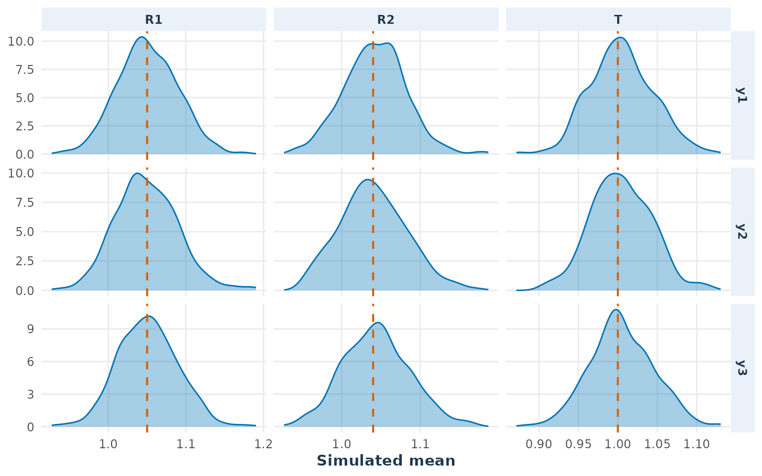

plot_distribution(ss_pilot, estimand = "sigma")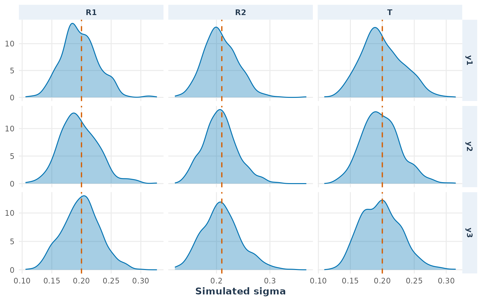

If the distributions are centered away from their references, check the input parameterization and the simulation code. If they are very wide, that may be expected for the pilot sample size; it is a precision issue, not necessarily a bias issue.

3b. Endpoint correlations

This plot checks whether the empirical within-arm endpoint correlations are centered near the specified value of 0.50. It checks dependence between endpoints in the same arm, not dependence between treatment arms.

plot_distribution(ss_pilot, estimand = "correlation")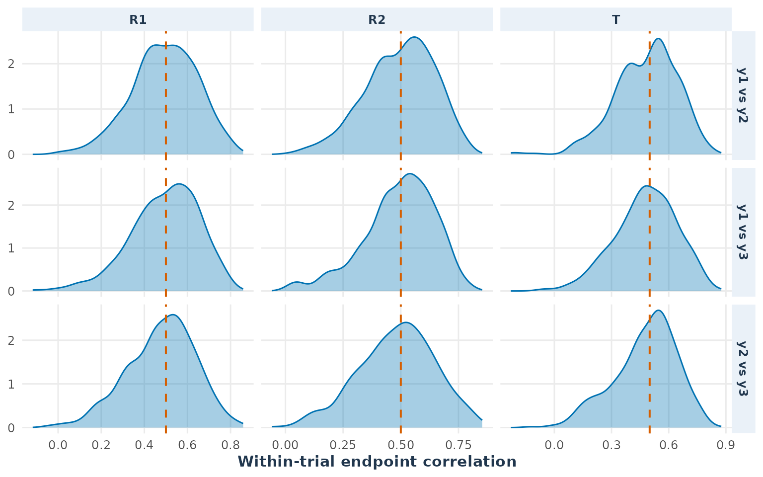

If the correlations are wrong, check rho or cor_mat, endpoint order, and the covariance construction. Do not interpret joint power until this check is satisfactory because endpoint correlation affects the probability that multiple endpoint tests pass together.

3c. Estimand direction and sampling distribution

This plot checks the quantity used by the test. Because the comparators are c(test, reference), the theoretical ROM values are approximately 0.95 for T_vs_R1 and 0.96 for T_vs_R2.

plot_distribution(ss_pilot, estimand = "ROM")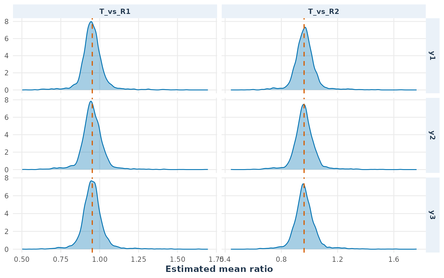

If the distribution is centered near the reciprocal, such as approximately 0.95 instead of 1.05, the comparator direction has been reversed. Correct list_comparator before continuing. A shift that is not a reciprocal usually indicates an issue with the supplied means or the ROM calculation.

3d. TOST t-statistics

You can also inspect the distributions of the two one-sided test statistics used by the TOST procedure:

plot_distribution(ss_pilot, estimand = "t_value",
                  arms = c("T", "R1", "R2"))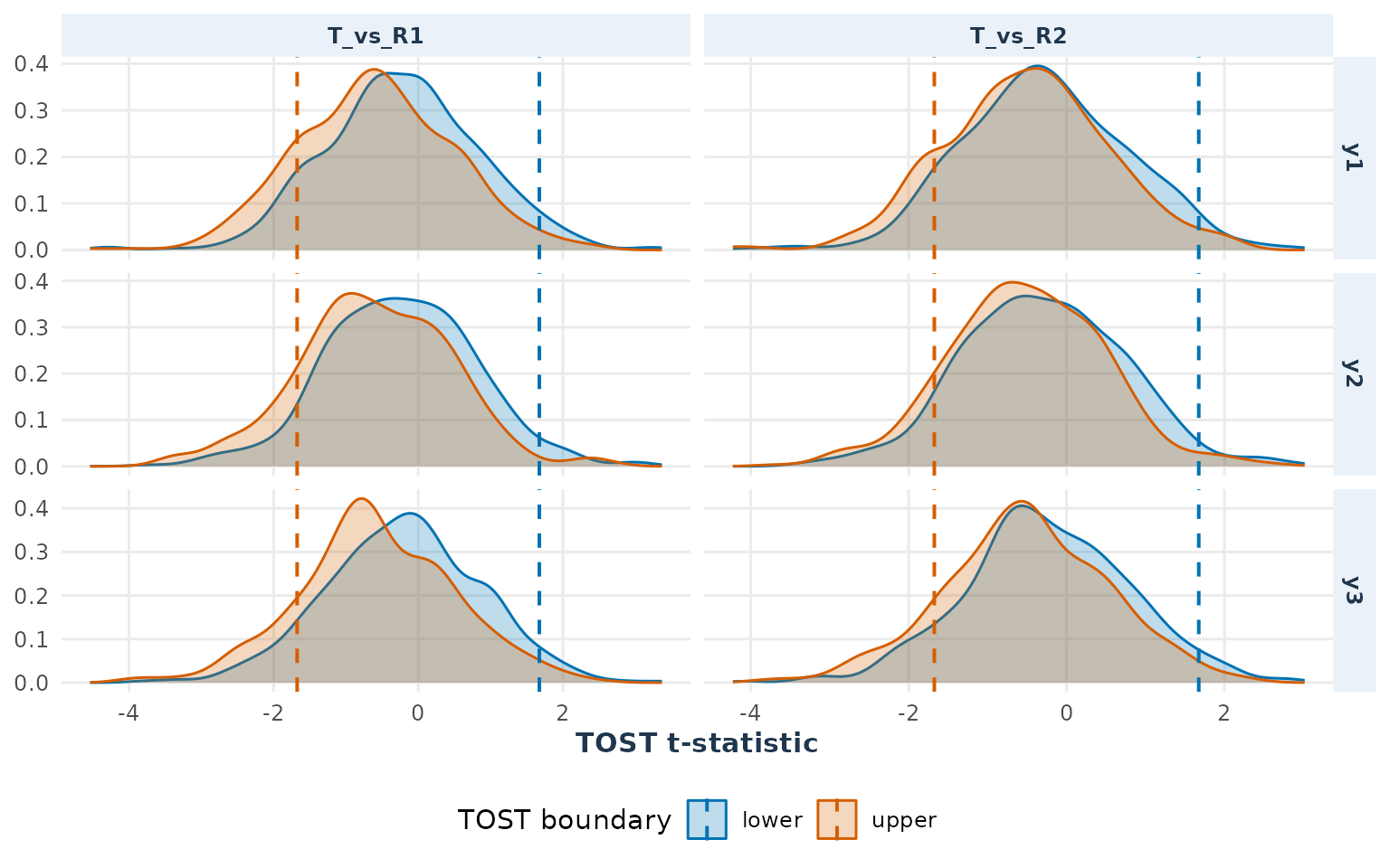

Each panel is one endpoint and comparator. The blue and orange curves are the lower-bound and upper-bound t-statistics. The dashed lines are their one-sided critical values. For an endpoint to pass equivalence, the lower statistic should be to the right of its critical line and the upper statistic should be to the left of its critical line. If one curve frequently lies on the wrong side, that boundary is responsible for many endpoint failures.

These t-statistics are reconstructed from the retained outcomes using the same continuous parallel-test formulas as the TOST calculation. They are a diagnostic of the statistic’s distribution, not a replacement for the trial-level decisions in plot_decision_heatmap() or the numerical power in summary(ss).

The n_trials argument used in the plots only limits the observations displayed. It is not the number of Monte Carlo trials used by the power calculation; that number is nsim.

Step 4: Check Monte Carlo stability and precision

This step addresses: “Is the number of simulations (nsim) sufficient for a stable estimate?” It assesses precision, not model validity or study sample size. Every simulation estimate has Monte Carlo uncertainty. Simulation-study guidance recommends reporting this uncertainty and choosing the number of repetitions to achieve a stated precision (Siepe et al. 2024).

The plot_stability() checks if the estimated rejection probability stabilizes as simulations accumulate. Compare the final value to the target power (0.80). By default, it diagnoses each comparator separately (overall = FALSE), use find which individual comparator or endpoint is causing instability. On the other hand use overall = TRUE for study-level precision checks, i.e to show the probability that the complete all-comparators decision passes in a trial.

plot_stability(ss_pilot, overall = TRUE)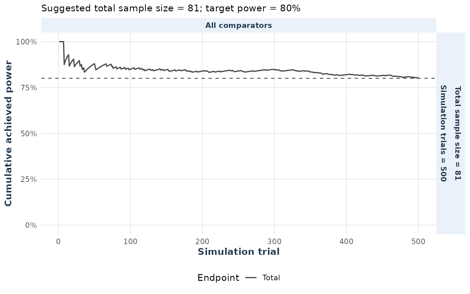

The plot_mc_error(): Displays the remaining Monte Carlo uncertainty around the power estimate. The title and labels above the final points show the achieved Monte Carlo error (half-width of the 95% confidence interval)

plot_mc_error(ss_pilot, overall = TRUE)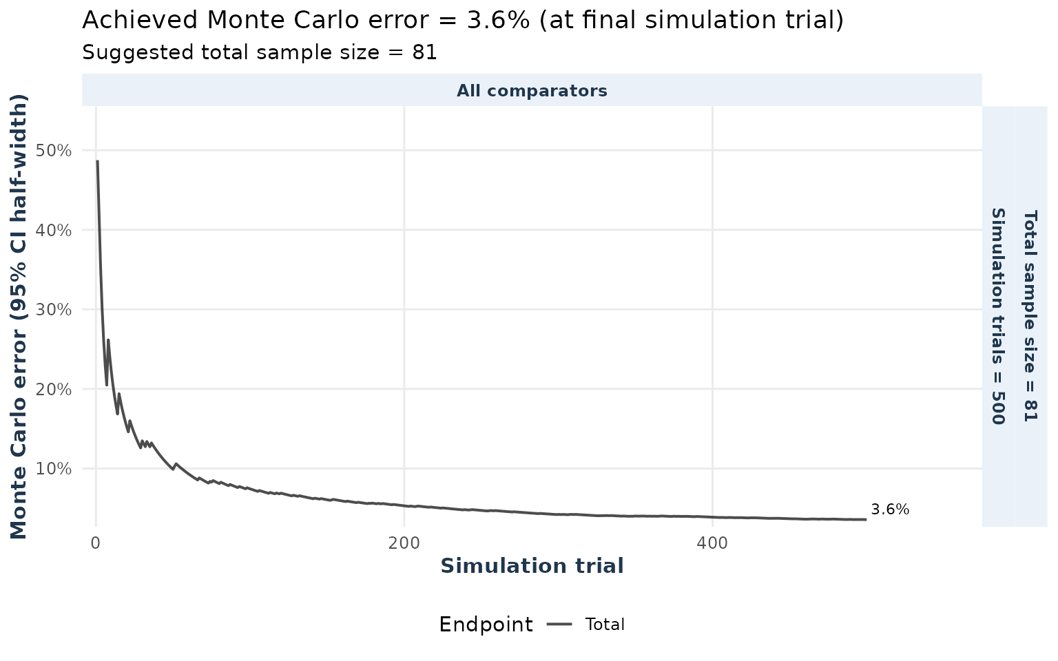

Here, you need to ensure the curve has broadly stabilized and inspect the displayed Monte Carlo error. If the error is too large for the desired precision, increase nsim. For example, an estimate of 0.80 [0.79, 0.81] (half-width ~0.01) meets a 1% precision criterion, while 0.80 [0.765, 0.835] (half-width ~0.035) does not. In the latter case, increase nsim—not the participant sample size.

Note: Small fluctuations in the curves are normal. Focus on the final confidence interval width and broad stabilization. If power is below the target power despite precision, increase the participant sample size. If checks fail, correct model inputs and rerun.

Step 5: Check Type I error at the equivalence boundaries

This step answers: “If the true estimand (in this example ratio of means (ROM)) is exactly at an equivalence boundary, how often does the study incorrectly conclude equivalence?”

One endpoint example

Let us start with a small example so the calculation is easy to see. Consider a trial with:

One comparator (T_vs_R1) and one endpoint (y1).
Estimand, ROM: $\theta = \frac{\mu_{T,y1}}{\mu_{R1,y1}}.$
Equivalence limits: Lower (L = 0.80) and upper (U = 1.25).
Equivalence condition: $L = 0.80, \qquad U = 1.25.$

The TOST (Two One-Sided Tests) decision requires rejecting both:

$H_{0L}: \theta \leq L \quad\text{versus}\quad H_{1L}: \theta > L,$ $H_{0U}: \theta \geq U \quad\text{versus}\quad H_{1U}: \theta < U.$

For a log-normal outcome with ctype = "ROM", the boundary is set on the log-analysis scale. Define

$\eta_a = \log(\mu_{a,y1}) - \frac{1}{2} \log\left(1 + \frac{\sigma_{a,y1}^2}{\mu_{a,y1}^2}\right),$

where $\eta_a$ is the log-analysis mean for arm $a$ .

For lower-boundary scenario, the function sets

$\exp(\eta_T - \eta_{R1}) = L = 0.80.$

With $\mu_{R1,y1} = 1.05$ and both standard deviations equal to 0.20, this corresponds approximately to

$\mu_{T,y1}=0.8478135, \qquad \frac{\mu_{T,y1}}{\mu_{R1,y1}}=0.8074414, \qquad \exp(\eta_T-\eta_{R1})=0.80.$

For the upper-boundary scenario, the function sets: $\exp(\eta_T - \eta_{R1}) = U = 1.25.$

For the same supplied reference mean and standard deviation, this gives approximately $\mu_{T,y1}=1.304387$ and an arithmetic mean ratio of 1.242273, while the log-analysis ROM is exactly 1.25.

A false-equivalence event occurs if the confidence interval for the estimated log-ratio falls within (log(0.80), log(1.25)) despite the true ROM being 0.80 or 1.25.

Particularly, the type1Error() function simulates each scenario individually, reporting the type I error, i.e. the probability that all required tests incorrectly conclude equivalence when the true effect is at the boundary of the acceptable range. For example, if a study requires three endpoints to pass equivalence tests, this error measures how often all three tests pass incorrectly at the boundary.

When applied to the simss object with null = "both", the function evaluates both the lower and upper boundaries separately. With joint = TRUE, it assesses every comparator–endpoint combination and reports the Type I error for the complete trial decision, using the stored k values.

The output table and plot display for each scenario the type I error along with 95% Monte Carlo confidence intervals.

ss_one <- sampleSize(
  power = 0.80, alpha = 0.05,
  mu_list = list(T = mu_t["y1"], R1 = mu_r1["y1"]),
  sigma_list = list(T = sigma_t["y1"], R1 = sigma_r1["y1"]),
  list_comparator = list(T_vs_R1 = c("T", "R1")),
  list_y_comparator = list(T_vs_R1 = "y1"),
  list_lequi.tol = list(T_vs_R1 = c(y1 = 0.80)),
  list_uequi.tol = list(T_vs_R1 = c(y1 = 1.25)),
  dtype = "parallel", distribution = "lnorm", ctype = "ROM",
  lower = 10, upper = 100, nsim = 1000, seed = 2026, ncores = 1
)
type1_one <- type1Error(x = ss_one, null = "both", joint = TRUE)
print(type1_one)
#> Joint empirical Type I error analysis
#> Boundary configurations: 2 
#>  Boundary Comparator Endpoint NullCount Type1_Error      Lower      Upper
#>     lower    T_vs_R1       y1         1        0.05 0.03769546 0.06587483
#>     upper    T_vs_R1       y1         1        0.04 0.02908471 0.05457906
#>  Simultaneous_Upper
#>          0.06539049
#>          0.05407270
#> Global worst-case Type I error: 0.0500 [0.0377, 0.0659]
#> Simultaneous 95.0% upper bound for global Type I error: 0.0654
#> Global scenario: T_vs_R1, y1, lower boundary
plot(type1_one)
#> Warning: Removed 1 row containing missing values or values outside the scale range
#> (`geom_point()`).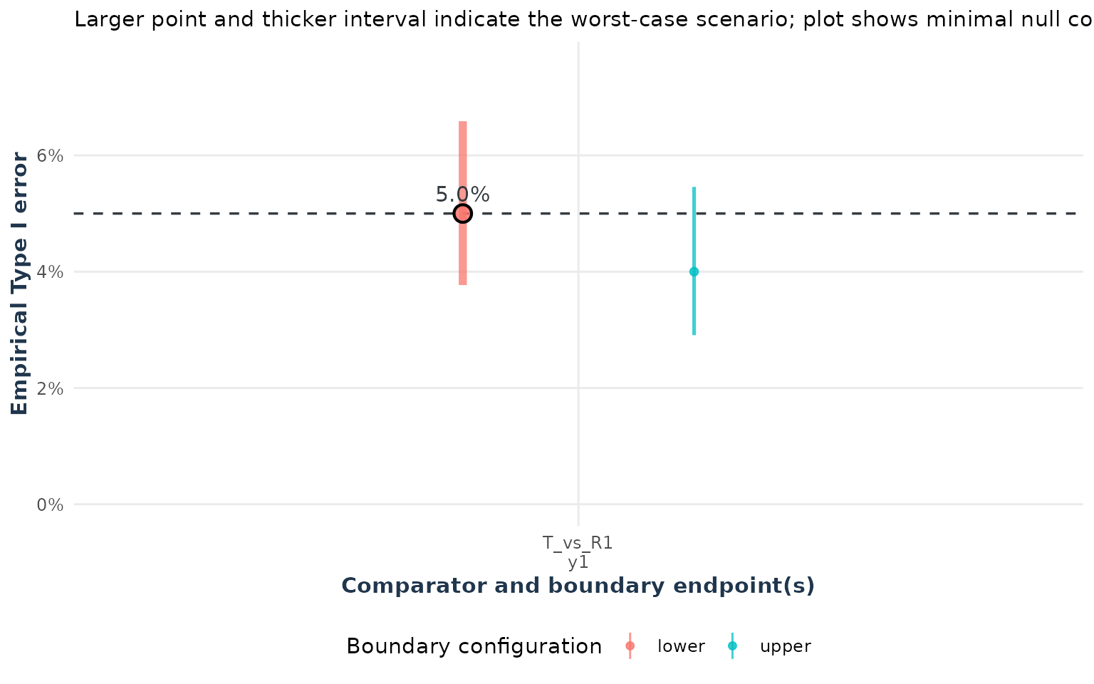

To estimate the global Type I error, use the least favorable scenario (the one with the highest type I error). In the plot, this scenario is highlighted with a thicker point and confidence line. The target quantity is

$\alpha_{\mathrm{global}} = \sup_{\theta \in H_0} P_{\theta}(\text{complete-trial success}),$

the highest probability of a false complete-trial conclusion over the null parameter space. This is the standard definition of the size of a test for a composite null hypothesis (Lehmann and Romano 2005, chap. 3). In this multiple-endpoint setting, the least-favorable-configuration literature applies the same principle by searching for the null configuration that maximizes the rejection probability (Ristl et al. 2019). In the one-endpoint example, the boundary scenarios are the complete null configuration.

The type1Error() function evaluates the prespecified boundary grid and reports the largest empirical complete-trial success probability as an approximation to the global Type I error; probabilities are therefore not averaged across scenarios. This is a finite-grid estimate, not a proof that the reported scenario is the supremum over all effect sizes and nuisance parameters.

Finally, compare the global Type I error point estimate and confidence interval against the nominal value (here 5%):

Contains the nominal value: Compatible with the nominal value at this simulation precision; this is not a formal calibration test.
Entirely above the nominal value: Evidence of possible global inflation, subject to Monte Carlo error and the adequacy of the scenario grid.
Entirely below the nominal value: Evidence of conservatism, subject to Monte Carlo error and the adequacy of the scenario grid.

Multiple endpoints example

The one-endpoint example is illustrative, but in more complex cases (e.g., the pilot example), the analysis extends to every endpoint in both comparisons and for both boundaries (lower and upper).

For multiple endpoints, the null configuration depends on the decision rule: when all endpoints are required (k = m), the global null is the union of the component nulls; when only k < m endpoints are required, it is a partial-conjunction null.

Ristl et al. (Ristl et al. 2019) describe the least-favorable-configuration principle for multiple endpoints. In the all-required case, a candidate least-favorable configuration has one component at its null boundary and the other components at favorable alternatives. For a k-of-m rule, the corresponding minimal null has $r = m - k + 1$ non-equivalent endpoints at boundaries and the remaining k - 1 endpoints at favorable alternatives.

For one fixed selected comparator, the number of configurations is ${m \choose r}2^{r}.$ Here, ${m \choose r}$ chooses the r boundary endpoints and $2^r$ chooses whether each boundary is lower (L) or upper (U). If the analysis has $q$ comparators and the grid repeats these configurations with each comparator selected in turn, the total number of configurations is $q {m \choose r}2^{r}.$ For example, with two comparators and three endpoints, this gives 12, 24, and 16 configurations for k = 3, k = 2, and k = 1, respectively. Additional nuisance-parameter values may be added for robustness. The configuration grid is a finite approximation to the null parameter space.

Particularly, for each scenario, the selected component is placed at its equivalence boundary, while other components are set at favorable alternatives, here the midpoint of their equivalence interval:

For continuous outcomes: (L + U) / 2 (difference) or sqrt(L * U) (ratio).
For log-normal ROM, the midpoint is converted to an arithmetic mean using variance-based calibration.
For Poisson and negative-binomial outcomes, sqrt(L * U) is used, but absolute rates, exposure, and dispersion (for negative binomial) affect precision.

The continuous-outcome midpoint is motivated by Anderson’s inequality: for a fixed-covariance Gaussian estimator, the probability of falling in a symmetric convex acceptance region is maximized when its mean is at the centre of that region (Anderson 1955). This gives (L + U) / 2 on a difference scale and sqrt(L * U) on a ratio scale, because the latter is the midpoint on the log-ratio scale. In a multiple-endpoint equivalence problem, this is used as a reproducible candidate configuration for the non-selected components, alongside the joint-equivalence framework described by Quan et al. (Quan et al. 2001). It is not a universal theorem for Poisson or negative-binomial models: their nuisance rates, exposure, and dispersion can change the joint probability, so those configurations may need an additional grid or optimization check.

The midpoint is a practical finite candidate for a favorable alternative, not a universal least-favorable result for Poisson or negative-binomial models. For count outcomes, the grid should be expanded over plausible rates, exposure, dispersion, and dependence values when those nuisance parameters could change the maximizing configuration.

`k = 3`: all endpoints are required

When k = m, the decision for the complete trial is an intersection–union test (IUT). For three endpoints and two comparisons, the trial passes only when

$D = (D_{R1,y1} \cap D_{R1,y2} \cap D_{R1,y3}) \cap (D_{R2,y1} \cap D_{R2,y2} \cap D_{R2,y3})$

is true. The global null is the union of the component nulls: at least one of the six component equivalence claims is false. Since the final decision requires an intersection of component decisions, testing each component TOST at level α does not require an additional endpoint-wise multiplicity correction in this all-required setting. This is the usual IUT logic for multiple-endpoint equivalence testing (Berger and Hsu 1996).

For k = 3, one endpoint is placed at a boundary. For T_vs_R1, the six configurations are

(L, M, M)  (U, M, M)
(M, L, M)  (M, U, M)
(M, M, L)  (M, M, U)

For each of these, the T_vs_R2 endpoints are (M, M, M). The same six configurations are then repeated with T_vs_R2 as the selected null comparator and T_vs_R1 equal to (M, M, M).

type1_global <- type1Error(x = ss_pilot, null = "both", joint = TRUE)
print(type1_global)
#> Joint empirical Type I error analysis
#> Boundary configurations: 52 
#>           Boundary Comparator Endpoint NullCount Type1_Error        Lower
#>              lower    T_vs_R1       y1         1       0.032 0.0190254452
#>              upper    T_vs_R1       y1         1       0.042 0.0268352453
#>              lower    T_vs_R1       y2         1       0.042 0.0268352453
#>              upper    T_vs_R1       y2         1       0.046 0.0300383801
#>              lower    T_vs_R1       y3         1       0.032 0.0190254452
#>              upper    T_vs_R1       y3         1       0.036 0.0221111654
#>              lower    T_vs_R1    y1+y2         2       0.008 0.0025657927
#>        upper/lower    T_vs_R1    y1+y2         2       0.000 0.0000000000
#>        lower/upper    T_vs_R1    y1+y2         2       0.000 0.0000000000
#>              upper    T_vs_R1    y1+y2         2       0.006 0.0015508542
#>              lower    T_vs_R1    y1+y3         2       0.006 0.0015508542
#>        upper/lower    T_vs_R1    y1+y3         2       0.000 0.0000000000
#>        lower/upper    T_vs_R1    y1+y3         2       0.000 0.0000000000
#>              upper    T_vs_R1    y1+y3         2       0.004 0.0006931365
#>              lower    T_vs_R1    y2+y3         2       0.008 0.0025657927
#>        upper/lower    T_vs_R1    y2+y3         2       0.000 0.0000000000
#>        lower/upper    T_vs_R1    y2+y3         2       0.000 0.0000000000
#>              upper    T_vs_R1    y2+y3         2       0.014 0.0061482689
#>              lower    T_vs_R1 y1+y2+y3         3       0.002 0.0001044091
#>  upper/lower/lower    T_vs_R1 y1+y2+y3         3       0.000 0.0000000000
#>  lower/upper/lower    T_vs_R1 y1+y2+y3         3       0.000 0.0000000000
#>  upper/upper/lower    T_vs_R1 y1+y2+y3         3       0.000 0.0000000000
#>  lower/lower/upper    T_vs_R1 y1+y2+y3         3       0.000 0.0000000000
#>  upper/lower/upper    T_vs_R1 y1+y2+y3         3       0.000 0.0000000000
#>  lower/upper/upper    T_vs_R1 y1+y2+y3         3       0.000 0.0000000000
#>              upper    T_vs_R1 y1+y2+y3         3       0.004 0.0006931365
#>              lower    T_vs_R2       y1         1       0.036 0.0221111654
#>              upper    T_vs_R2       y1         1       0.034 0.0205612556
#>              lower    T_vs_R2       y2         1       0.046 0.0300383801
#>              upper    T_vs_R2       y2         1       0.046 0.0300383801
#>              lower    T_vs_R2       y3         1       0.040 0.0252490565
#>              upper    T_vs_R2       y3         1       0.024 0.0130517839
#>              lower    T_vs_R2    y1+y2         2       0.008 0.0025657927
#>        upper/lower    T_vs_R2    y1+y2         2       0.000 0.0000000000
#>        lower/upper    T_vs_R2    y1+y2         2       0.000 0.0000000000
#>              upper    T_vs_R2    y1+y2         2       0.014 0.0061482689
#>              lower    T_vs_R2    y1+y3         2       0.008 0.0025657927
#>        upper/lower    T_vs_R2    y1+y3         2       0.000 0.0000000000
#>        lower/upper    T_vs_R2    y1+y3         2       0.000 0.0000000000
#>              upper    T_vs_R2    y1+y3         2       0.006 0.0015508542
#>              lower    T_vs_R2    y2+y3         2       0.008 0.0025657927
#>        upper/lower    T_vs_R2    y2+y3         2       0.000 0.0000000000
#>        lower/upper    T_vs_R2    y2+y3         2       0.000 0.0000000000
#>              upper    T_vs_R2    y2+y3         2       0.010 0.0036873010
#>              lower    T_vs_R2 y1+y2+y3         3       0.004 0.0006931365
#>  upper/lower/lower    T_vs_R2 y1+y2+y3         3       0.000 0.0000000000
#>  lower/upper/lower    T_vs_R2 y1+y2+y3         3       0.000 0.0000000000
#>  upper/upper/lower    T_vs_R2 y1+y2+y3         3       0.000 0.0000000000
#>  lower/lower/upper    T_vs_R2 y1+y2+y3         3       0.000 0.0000000000
#>  upper/lower/upper    T_vs_R2 y1+y2+y3         3       0.000 0.0000000000
#>  lower/upper/upper    T_vs_R2 y1+y2+y3         3       0.000 0.0000000000
#>              upper    T_vs_R2 y1+y2+y3         3       0.008 0.0025657927
#>        Upper Simultaneous_Upper
#>  0.052559878         0.06430578
#>  0.064536740         0.07745598
#>  0.064536740         0.07745598
#>  0.069253580         0.08259568
#>  0.052559878         0.06430578
#>  0.057386056         0.06962373
#>  0.021799801         0.02937247
#>  0.009504683         0.01379788
#>  0.009504683         0.01379788
#>  0.018951807         0.02596010
#>  0.018951807         0.02596010
#>  0.009504683         0.01379788
#>  0.009504683         0.01379788
#>  0.015997243         0.02234328
#>  0.021799801         0.02937247
#>  0.009504683         0.01379788
#>  0.009504683         0.01379788
#>  0.029937173         0.03887309
#>  0.012885458         0.01840095
#>  0.009504683         0.01379788
#>  0.009504683         0.01379788
#>  0.009504683         0.01379788
#>  0.009504683         0.01379788
#>  0.009504683         0.01379788
#>  0.009504683         0.01379788
#>  0.015997243         0.02234328
#>  0.057386056         0.06962373
#>  0.054979471         0.06697541
#>  0.069253580         0.08259568
#>  0.069253580         0.08259568
#>  0.062163899         0.07486270
#>  0.042726845         0.05337262
#>  0.021799801         0.02937247
#>  0.009504683         0.01379788
#>  0.009504683         0.01379788
#>  0.029937173         0.03887309
#>  0.021799801         0.02937247
#>  0.009504683         0.01379788
#>  0.009504683         0.01379788
#>  0.018951807         0.02596010
#>  0.021799801         0.02937247
#>  0.009504683         0.01379788
#>  0.009504683         0.01379788
#>  0.024569311         0.03264068
#>  0.015997243         0.02234328
#>  0.009504683         0.01379788
#>  0.009504683         0.01379788
#>  0.009504683         0.01379788
#>  0.009504683         0.01379788
#>  0.009504683         0.01379788
#>  0.009504683         0.01379788
#>  0.021799801         0.02937247
#> Global worst-case Type I error: 0.0460 [0.0300, 0.0693]
#> Simultaneous 95.0% upper bound for global Type I error: 0.0826
#> Global scenario: T_vs_R1, y2, upper boundary
plot(type1_global)
#> Warning: Removed 11 rows containing missing values or values outside the scale range
#> (`geom_point()`).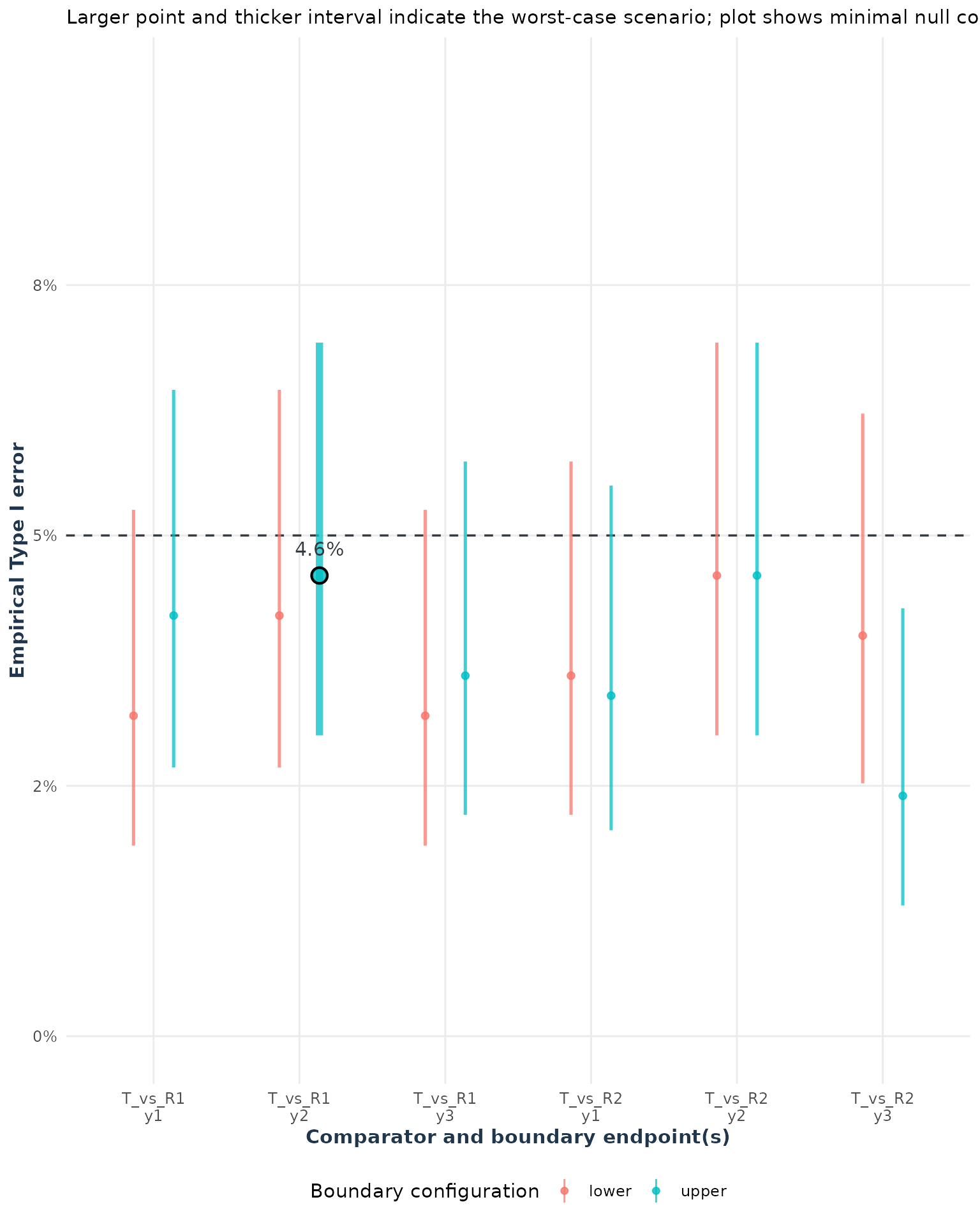

The corresponding simulated error is the probability that the complete trial decision passes, not merely the probability that the boundary component passes.

`k = 2`: at least two endpoints are required

The claim is that at least two of three endpoints are equivalent. This is a partial-conjunction rule, not the all-required IUT. Its null requires at least $r = 3 - 2 + 1 = 2$ non-equivalent endpoints. Therefore, for T_vs_R1, the 12 candidate configurations are

(L, L, M)  (L, U, M)  (U, L, M)  (U, U, M)
(L, M, L)  (L, M, U)  (U, M, L)  (U, M, U)
(M, L, L)  (M, L, U)  (M, U, L)  (M, U, U)

In each case, T_vs_R2 is (M, M, M). Repeating the 12 configurations with T_vs_R2 selected gives

$2\times {3\choose2}\times 2^2=24\ \text{scenarios}.$

Because the decision is “at least two,” a false claim can occur when an interior endpoint passes and one of the two boundary endpoints passes falsely. Therefore, an endpoint-wise multiplicity adjustment is needed for k < m; adjust = "bon" is a conservative starting point, and the complete-trial Type I error must be checked empirically (Benjamini and Heller 2008).

type1_global_k2 <- type1Error(x = ss_pilot_k2, null = "both", joint = TRUE)
#> Warning: The adjustment is applied within each comparator's selected endpoint
#> family, not across comparators; the global decision requires all comparator
#> decisions to pass.
print(type1_global_k2)
#> Joint empirical Type I error analysis
#> Boundary configurations: 40 
#>           Boundary Comparator Endpoint NullCount Type1_Error        Lower
#>              lower    T_vs_R1    y1+y2         2       0.016 0.0074584371
#>        upper/lower    T_vs_R1    y1+y2         2       0.030 0.0175049931
#>        lower/upper    T_vs_R1    y1+y2         2       0.018 0.0088094113
#>              upper    T_vs_R1    y1+y2         2       0.024 0.0130517839
#>              lower    T_vs_R1    y1+y3         2       0.010 0.0036873010
#>        upper/lower    T_vs_R1    y1+y3         2       0.014 0.0061482689
#>        lower/upper    T_vs_R1    y1+y3         2       0.022 0.0116103433
#>              upper    T_vs_R1    y1+y3         2       0.026 0.0145162787
#>              lower    T_vs_R1    y2+y3         2       0.008 0.0025657927
#>        upper/lower    T_vs_R1    y2+y3         2       0.024 0.0130517839
#>        lower/upper    T_vs_R1    y2+y3         2       0.038 0.0236740836
#>              upper    T_vs_R1    y2+y3         2       0.036 0.0221111654
#>              lower    T_vs_R1 y1+y2+y3         3       0.000 0.0000000000
#>  upper/lower/lower    T_vs_R1 y1+y2+y3         3       0.000 0.0000000000
#>  lower/upper/lower    T_vs_R1 y1+y2+y3         3       0.000 0.0000000000
#>  upper/upper/lower    T_vs_R1 y1+y2+y3         3       0.002 0.0001044091
#>  lower/lower/upper    T_vs_R1 y1+y2+y3         3       0.000 0.0000000000
#>  upper/lower/upper    T_vs_R1 y1+y2+y3         3       0.002 0.0001044091
#>  lower/upper/upper    T_vs_R1 y1+y2+y3         3       0.012 0.0048872944
#>              upper    T_vs_R1 y1+y2+y3         3       0.012 0.0048872944
#>              lower    T_vs_R2    y1+y2         2       0.030 0.0175049931
#>        upper/lower    T_vs_R2    y1+y2         2       0.030 0.0175049931
#>        lower/upper    T_vs_R2    y1+y2         2       0.036 0.0221111654
#>              upper    T_vs_R2    y1+y2         2       0.026 0.0145162787
#>              lower    T_vs_R2    y1+y3         2       0.030 0.0175049931
#>        upper/lower    T_vs_R2    y1+y3         2       0.030 0.0175049931
#>        lower/upper    T_vs_R2    y1+y3         2       0.024 0.0130517839
#>              upper    T_vs_R2    y1+y3         2       0.022 0.0116103433
#>              lower    T_vs_R2    y2+y3         2       0.030 0.0175049931
#>        upper/lower    T_vs_R2    y2+y3         2       0.038 0.0236740836
#>        lower/upper    T_vs_R2    y2+y3         2       0.026 0.0145162787
#>              upper    T_vs_R2    y2+y3         2       0.026 0.0145162787
#>              lower    T_vs_R2 y1+y2+y3         3       0.010 0.0036873010
#>  upper/lower/lower    T_vs_R2 y1+y2+y3         3       0.006 0.0015508542
#>  lower/upper/lower    T_vs_R2 y1+y2+y3         3       0.002 0.0001044091
#>  upper/upper/lower    T_vs_R2 y1+y2+y3         3       0.002 0.0001044091
#>  lower/lower/upper    T_vs_R2 y1+y2+y3         3       0.004 0.0006931365
#>  upper/lower/upper    T_vs_R2 y1+y2+y3         3       0.006 0.0015508542
#>  lower/upper/upper    T_vs_R2 y1+y2+y3         3       0.004 0.0006931365
#>              upper    T_vs_R2 y1+y2+y3         3       0.008 0.0025657927
#>        Upper Simultaneous_Upper
#>  0.032555702         0.04108766
#>  0.050126186         0.06069039
#>  0.035139646         0.04400921
#>  0.042726845         0.05250261
#>  0.024569311         0.03192777
#>  0.029937173         0.03810837
#>  0.040221837         0.04971085
#>  0.045211262         0.05526091
#>  0.021799801         0.02868876
#>  0.042726845         0.05250261
#>  0.059780585         0.07126775
#>  0.057386056         0.06865388
#>  0.009504683         0.01328025
#>  0.009504683         0.01328025
#>  0.009504683         0.01328025
#>  0.012885458         0.01782873
#>  0.009504683         0.01328025
#>  0.012885458         0.01782873
#>  0.027277839         0.03506020
#>  0.027277839         0.03506020
#>  0.050126186         0.06069039
#>  0.050126186         0.06069039
#>  0.057386056         0.06865388
#>  0.045211262         0.05526091
#>  0.050126186         0.06069039
#>  0.050126186         0.06069039
#>  0.042726845         0.05250261
#>  0.040221837         0.04971085
#>  0.050126186         0.06069039
#>  0.059780585         0.07126775
#>  0.045211262         0.05526091
#>  0.045211262         0.05526091
#>  0.024569311         0.03192777
#>  0.018951807         0.02530864
#>  0.012885458         0.01782873
#>  0.012885458         0.01782873
#>  0.015997243         0.02172827
#>  0.018951807         0.02530864
#>  0.015997243         0.02172827
#>  0.021799801         0.02868876
#> Global worst-case Type I error: 0.0380 [0.0237, 0.0598]
#> Simultaneous 95.0% upper bound for global Type I error: 0.0713
#> Global scenario: T_vs_R1, y2+y3, lower/upper boundary
plot(type1_global_k2)
#> Warning: Removed 23 rows containing missing values or values outside the scale range
#> (`geom_point()`).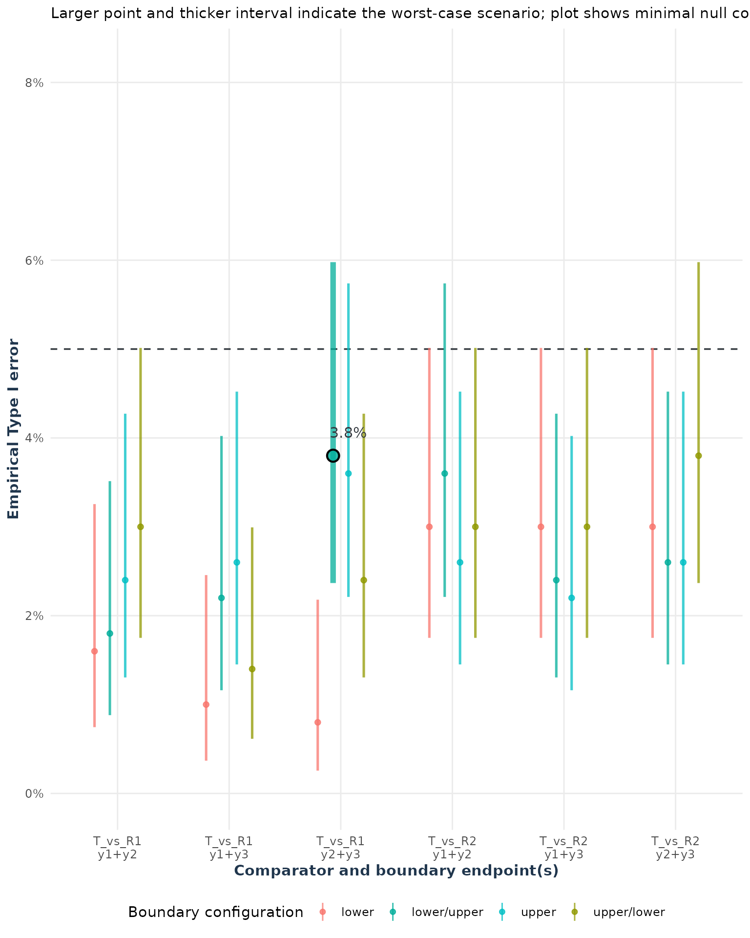

The default joint plot displays only the minimal null configurations, with m - k + 1 boundary endpoints (two endpoints here). The numerical global Type I error still uses the complete grid, including configurations with three boundary endpoints. To display every evaluated configuration, use plot(type1_global_k2, null_count = "all").

`k = 1`: at least one endpoint is required

The claim is that at least one endpoint is equivalent. Its null requires all three endpoints to be non-equivalent, so $r = 3 - 1 + 1 = 3$ . For T_vs_R1, the eight candidate configurations are

(L, L, L)  (L, L, U)  (L, U, L)  (L, U, U)
(U, L, L)  (U, L, U)  (U, U, L)  (U, U, U)

In each case, T_vs_R2 is (M, M, M). Repeating these eight configurations with T_vs_R2 selected gives

$2\times {3\choose3}\times 2^3=16\ \text{scenarios}.$

type1_global_k1 <- type1Error(x = ss_pilot_k1, null = "both", joint = TRUE)
#> Warning: The adjustment is applied within each comparator's selected endpoint
#> family, not across comparators; the global decision requires all comparator
#> decisions to pass.
print(type1_global_k1)
#> Joint empirical Type I error analysis
#> Boundary configurations: 16 
#>           Boundary Comparator Endpoint NullCount Type1_Error       Lower
#>              lower    T_vs_R1 y1+y2+y3         3       0.014 0.006148269
#>  upper/lower/lower    T_vs_R1 y1+y2+y3         3       0.040 0.025249056
#>  lower/upper/lower    T_vs_R1 y1+y2+y3         3       0.038 0.023674084
#>  upper/upper/lower    T_vs_R1 y1+y2+y3         3       0.054 0.036551387
#>  lower/lower/upper    T_vs_R1 y1+y2+y3         3       0.040 0.025249056
#>  upper/lower/upper    T_vs_R1 y1+y2+y3         3       0.056 0.038199110
#>  lower/upper/upper    T_vs_R1 y1+y2+y3         3       0.056 0.038199110
#>              upper    T_vs_R1 y1+y2+y3         3       0.064 0.044856884
#>              lower    T_vs_R2 y1+y2+y3         3       0.038 0.023674084
#>  upper/lower/lower    T_vs_R2 y1+y2+y3         3       0.060 0.041515247
#>  lower/upper/lower    T_vs_R2 y1+y2+y3         3       0.056 0.038199110
#>  upper/upper/lower    T_vs_R2 y1+y2+y3         3       0.062 0.043183022
#>  lower/lower/upper    T_vs_R2 y1+y2+y3         3       0.044 0.028431907
#>  upper/lower/upper    T_vs_R2 y1+y2+y3         3       0.056 0.038199110
#>  lower/upper/upper    T_vs_R2 y1+y2+y3         3       0.048 0.031654072
#>              upper    T_vs_R2 y1+y2+y3         3       0.054 0.036551387
#>       Upper Simultaneous_Upper
#>  0.02993717         0.03537130
#>  0.06216390         0.07025447
#>  0.05978059         0.06771179
#>  0.07858655         0.08767767
#>  0.06216390         0.07025447
#>  0.08090132         0.09012174
#>  0.08090132         0.09012174
#>  0.09009660         0.09980682
#>  0.05978059         0.06771179
#>  0.08551115         0.09498168
#>  0.08090132         0.09012174
#>  0.08780679         0.09739841
#>  0.06689977         0.07529539
#>  0.08090132         0.09012174
#>  0.07159870         0.08028309
#>  0.07858655         0.08767767
#> Global worst-case Type I error: 0.0640 [0.0449, 0.0901]
#> Simultaneous 95.0% upper bound for global Type I error: 0.0998
#> Global scenario: T_vs_R1, y1+y2+y3, upper boundary
plot(type1_global_k1)
#> Warning: Removed 15 rows containing missing values or values outside the scale range
#> (`geom_point()`).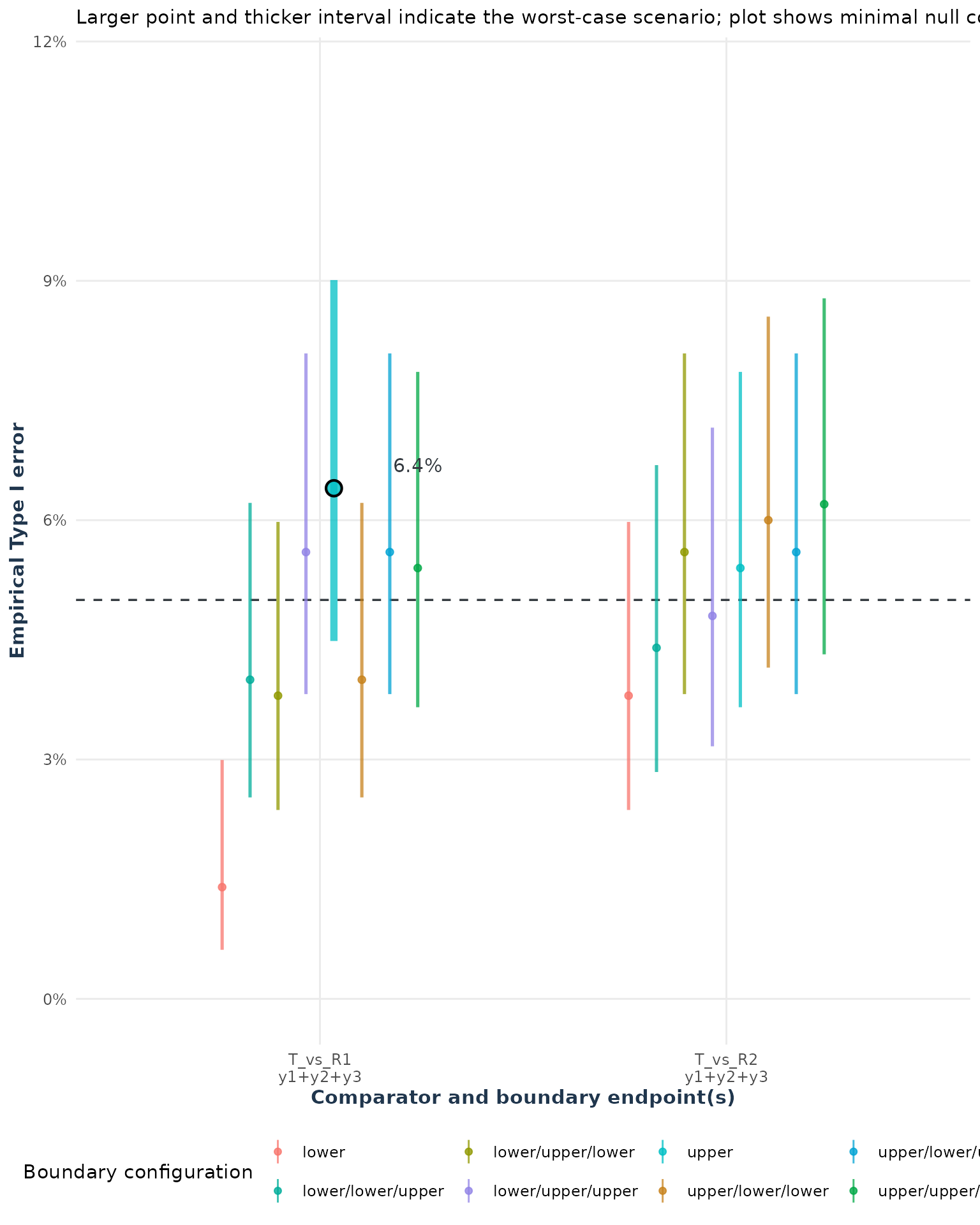

This is the most permissive rule: any one boundary endpoint passing falsely can complete the claim. A multiplicity adjustment is therefore essential, and the global result should be checked using the largest joint Type I-error estimate and its Monte Carlo interval.

For every configuration above, the simulated trial must satisfy the complete study decision: the required number of endpoints must pass for T_vs_R1 and for T_vs_R2 in the same trial.

The reported global Type I error is an empirical approximation of the worst-case scenario among the evaluated boundary configurations. Compare the global interval to the nominal value (5%) line as we did in the previous section.

For k = m, adjust = "no" is generally appropriate for the endpoint IUT. For k < m, use Mielke’s strong adjust = "t" calibration alpha / (m - k + 1) when strong control over partial null configurations is required. The package’s adjust = "k" method uses k * alpha / m and is a weak complete-null calibration; it should be used only when that estimand is the prespecified objective. Confirm the global performance with type1Error().

Step 6: Run the final sample-size calculation

Only after the pilot has passed the distribution, estimand, correlation, Monte Carlo, and Type I-error checks should the model be used for final planning. The final call can use a larger nsim than the pilot. Retaining raw data is optional at this stage; it is useful if the final result also needs an audit trail of simulated outcomes.

ss <- sampleSize(
  power = 0.80, alpha = 0.05,
  mu_list = list(T = mu_t, R1 = mu_r1, R2 = mu_r2),
  sigma_list = list(T = sigma_t, R1 = sigma_r1, R2 = sigma_r2),
  rho = 0.50, list_comparator = comparators,
  list_y_comparator = list(T_vs_R1 = endpoints, T_vs_R2 = endpoints),
  list_lequi.tol = lower, list_uequi.tol = upper,
  dtype = "parallel", ctype = "ROM", distribution = "lnorm",
  adjust = "no", k = 3, ncores = 1, nsim = 2000, seed = 2026,
  keep_sim_data = TRUE
)

In this example, the final run uses more trials than the 500-trial pilot. If the final power decision is close to 0.80, increase this to 5,000 trials and use the final value displayed by plot_mc_error(ss) as a stricter precision check. The appropriate choice is the smallest nsim that gives a stable estimate and a confidence interval narrow enough for the planned conclusion.

Step 7: Interpret and report the final result

Now inspect the proposed sample size, achieved power, and Monte Carlo interval. For a parallel design, n is the base sample size used to derive the arm allocations; the summary also reports the total sample size.

print(ss)
#> Sample Size Calculation Results
#> -------------------------------------------------------------
#> Study Design: parallel trial targeting 80% power with a 5% type-I error.
#> 
#> Comparisons:
#>    T vs. R1 
#>     - Endpoints Tested: y1, y2, y3 
#>       (multiple co-primary endpoints, m =  3 )
#>    T vs. R2 
#>     - Endpoints Tested: y1, y2, y3 
#>       (multiple co-primary endpoints, m =  3 )
#> -------------------------------------------------------------
#>                  Parameter     Value
#>          Total Sample Size        81
#>             Achieved Power      81.4
#>  Power Confidence Interval 79.6 - 83
#> -------------------------------------------------------------
summary(ss)
#> Sample Size Summary
#> ---------------------- 
#> Design type        : parallel 
#> Distribution       : lnorm 
#> Comparison type    : ROM 
#> Estimand           : arithmetic mean ratio
#> Hypotheses         : H0: ratio <= L or >= U; H1: L < ratio < U (tested on the log scale)
#> Alpha              : 0.05 
#> Target power       : 0.8000 
#> Achieved power     : 0.8135 
#> 
#> Equivalence Margins:
#>  Comparison Endpoint Lower Upper
#>     T_vs_R1       y1   0.8  1.25
#>     T_vs_R1       y2   0.8  1.25
#>     T_vs_R1       y3   0.8  1.25
#>     T_vs_R2       y1   0.8  1.25
#>     T_vs_R2       y2   0.8  1.25
#>     T_vs_R2       y3   0.8  1.25
#> 
#> Estimated Sample Size:
#>  n_T n_R1 n_R2 n_total
#>   27   27   27      81
confint(ss)
#> Confidence Interval for Achieved Power (95%):
#>  0.8135 [0.7956, 0.8302]
plot(ss)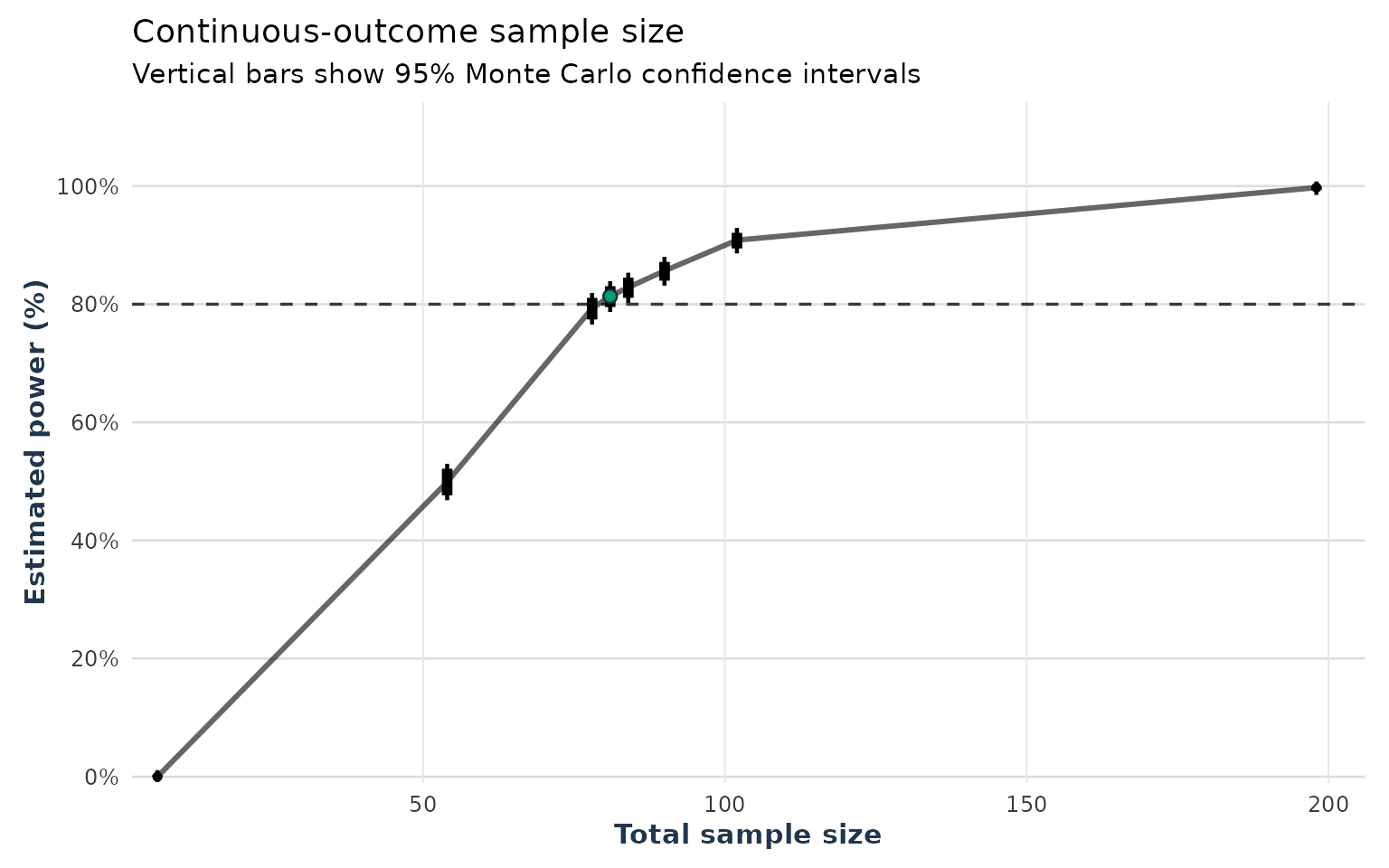

The result is acceptable only if the model checks passed, the Monte Carlo interval is sufficiently narrow, the Type I-error assessment is reasonable, and achieved power is close to the target. If the final power is too low or too imprecise, increase the planned sample size or nsim as appropriate. If it differs because a diagnostic failed, correct the model inputs and rerun the full workflow rather than simply increasing the sample size.

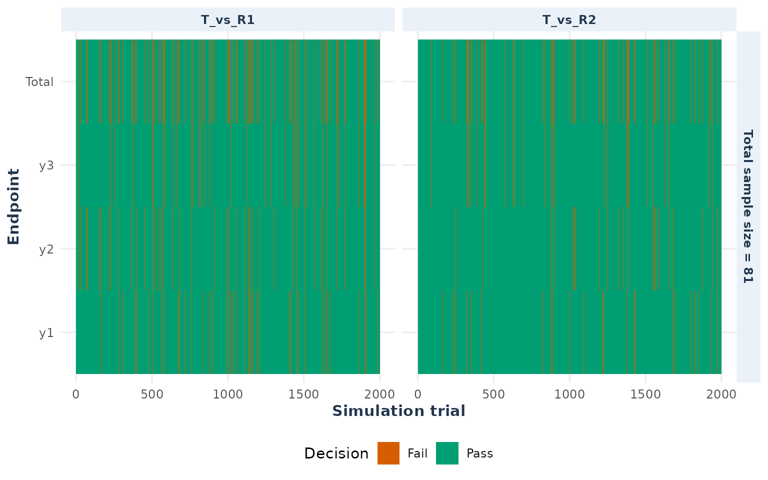
Finally, inspect endpoint-level decisions to identify which endpoint or comparison drives failures of the global rule. This is a diagnostic for the final result, not a replacement for the joint power or Type I-error assessment.

In addition, the plot_decision_heatmap() helps identify which endpoints or comparisons cause failures in the global decision rule by visualizing pass (green) or fail (orange) results for each simulated trial. Each row represents an endpoint, each facet a comparator (e.g., T_vs_R1), and the Total row shows the combined decision for that comparator—green only if all required endpoints pass. If a specific endpoint or comparator has more orange cells, it may be the bottleneck. Use this alongside summary(ss) and plot(ss): the summary provides numerical power, while the heatmap highlights which endpoints or comparisons are failing. Isolated orange cells are normal, but persistent bands indicate systematic issues.

plot_decision_heatmap(ss, display = c("T_vs_R1", "T_vs_R2"))

References

Anderson, T. W. 1955. “The Integral of a Symmetric Unimodal Function over a Symmetric Convex Set and Some Probability Inequalities.” Proceedings of the American Mathematical Society 6: 170–76. https://doi.org/10.1090/S0002-9939-1955-0069229-1.

Benjamini, Yoav, and Ruth Heller. 2008. “Screening for Partial Conjunction Hypotheses.” Biometrics 64 (4): 1215–22. https://doi.org/10.1111/j.1541-0420.2007.00984.x.

Berger, Roger L., and Jason C. Hsu. 1996. “Bioequivalence Trials, Intersection-Union Tests and Equivalence Confidence Sets.” Statistical Science 11 (4): 283–319. https://doi.org/10.1214/ss/1032280304.

Lehmann, Erich L., and Joseph P. Romano. 2005. Testing Statistical Hypotheses. 3rd ed. Springer Texts in Statistics. Springer. https://doi.org/10.1007/0-387-27605-X.

Quan, Hong, John Bolognese, and Wei Yuan. 2001. “Assessment of Equivalence on Multiple Endpoints.” Statistics in Medicine 20 (21): 3159–73. https://doi.org/10.1002/sim.985.

Ristl, Robin, Susanne Urach, Gerd Rosenkranz, and Martin Posch. 2019. “Methods for the Analysis of Multiple Endpoints in Small Populations: A Review.” Journal of Biopharmaceutical Statistics 29 (1): 1–29. https://doi.org/10.1080/10543406.2018.1489402.

Siepe, Björn S., František Bartoš, Tim P. Morris, Anne-Laure Boulesteix, Daniel W. Heck, and Samuel Pawel. 2024. “Simulation Studies for Methodological Research in Psychology: A Standardized Template for Planning, Preregistration, and Reporting.” Psychological Methods, ahead of print. https://doi.org/10.1037/met0000695.