Count Outcomes

Overview

This vignette follows the workflow in workflow.Rmd for count outcomes. It starts with a published two-arm Poisson benchmark, then validates a two-endpoint Poisson model, calculates its required sample size, repeats the calculation under a negative-binomial model, and finally uses the same model settings for a balanced two-by-two crossover design.

For count outcomes, the estimand is the event-rate ratio

$RR = \frac{\lambda_T}{\lambda_R},$

where the first arm in each comparator is the test arm and the second is the reference arm. Equivalence is assessed using two one-sided tests on the log-rate-ratio scale. The workflow separates model validation from the final equivalence calculation: first check the supplied parameters and retained simulated data, then calculate and interpret the sample size.

Parameters required for count outcomes

Count models require an event rate for every arm and endpoint, rather than a mean and standard deviation as in a continuous-outcome model. The main inputs are:

rate_list: the event rate for each arm, expressed per unit of exposure;
exposure: the amount of observation time or opportunity contributed by one participant;
list_comparator: the arm pairs to compare;
list_lequi.tol and list_uequi.tol: the lower and upper rate-ratio equivalence margins;
cor_mat: the dependence between endpoints when there is more than one endpoint; and
distribution: either "pois" for Poisson counts or "nbinom" for negative-binomial counts.

The expected count is the rate multiplied by the exposure:

$E(Y) = \text{rate} \times \text{exposure}.$

For example, a rate of 0.20 per week and an exposure of 10 weeks imply an expected count of 2 events per participant. In this example, exposure is not the number of participants; instead, it is the number of follow-up weeks. If the supplied rate is already an expected count per participant over the complete study period, use exposure = 1. The rate and exposure must use compatible time units. Exposure can be a scalar, an endpoint-specific vector, or arm-specific values when follow-up differs between arms.

For a Poisson model, the variance equals the mean and no dispersion parameter is needed. A negative-binomial model is used when the observed counts are more variable than a Poisson model allows. It requires the additional argument dispersion, which controls the extra variability while leaving the expected count unchanged:

$\operatorname{Var}(Y) = \mu + \text{dispersion}\,\mu^2, \qquad \mu = \text{rate} \times \text{exposure}.$

Thus, with an expected count of 2, dispersion = 0.50 gives a variance of approximately 2 + 0.50 * 2^2 = 4. Larger dispersion means more variation between participants and usually less information per participant, which can increase the required sample size. The dispersion should be chosen from pilot data or prior knowledge and examined in a sensitivity analysis; it is not a replacement for the event rate or the exposure. Poisson and negative-binomial rate equivalence planning is described by Chang et al. and Zhu (Chang et al. 2017; Zhu 2017).

The remaining planning inputs have the same meaning as for continuous outcomes: power, alpha, nsim, seed, and dtype specify the target power, type-I error level, number of simulations, reproducibility, and study design, respectively.

A published Poisson benchmark

Zhu (Zhu 2017) reports a two-arm Poisson equivalence calculation with equal event rates of 1 per time unit, average exposure of 0.7, equivalence limits of 0.9 and $1/0.9$ , one-sided $\alpha=0.025$ , and 2,705 participants per arm. The reported total sample size is 5,410, with approximated power 0.80012.

zhu_benchmark <- simPower(
  n = 2705,
  distribution = "pois",
  rate_list = list(TEST = 1, REF = 1),
  list_comparator = list(TEST_vs_REF = c("TEST", "REF")),
  list_lequi.tol = list(TEST_vs_REF = 0.9),
  list_uequi.tol = list(TEST_vs_REF = 1 / 0.9),
  exposure = 0.7,
  dtype = "parallel",
  alpha = 0.025,
  nsim = 5000,
  seed = 2024
)
zhu_benchmark
#> Fixed-sample-size power
#> Distribution: pois 
#> Sample size: 2705 
#> Power: 0.7936 [0.7821, 0.8047]
data.frame(reference_power = 0.80012,
           simulated_power = zhu_benchmark$power,
           simulated_lower = zhu_benchmark$power_LCI,
           simulated_upper = zhu_benchmark$power_UCI)
#>   reference_power simulated_power simulated_lower simulated_upper
#> 1         0.80012          0.7936       0.7820566       0.8046886

The simulation need not reproduce the published value exactly. The published result is a large-sample approximation, whereas simPower() simulates discrete event totals and reports a finite-sample Monte Carlo estimate.

A count outcome study example

Step 1: Define the study and theoretical targets

For this example, we utilize a two-endpoint, two-comparator count outcome study, which will serve as the foundation for the remainder of this vignette. The supplied endpoint correlation is a latent Gaussian-copula correlation, not the expected Pearson correlation of the observed counts (Nelsen 2006).

count_corr <- matrix(c(1, 0.5, 0.5, 1), nrow = 2,
                     dimnames = list(c("y1", "y2"), c("y1", "y2")))
count_rates <- list(TEST = c(y1 = 0.21, y2 = 0.24),
                    REF = c(y1 = 0.20, y2 = 0.22))
count_comparators <- list(TEST_vs_REF = c("TEST", "REF"))
count_lower <- list(TEST_vs_REF = c(y1 = 0.80, y2 = 0.80))
count_upper <- list(TEST_vs_REF = c(y1 = 1.25, y2 = 1.25))
count_exposure <- 10

Step 2: Run a pilot with `sampleSize()`

As in the workflow vignette, begin by running a pilot sample size calculation while retaining the simulated data. This object will be used for the diagnostics in the subsequent steps.

poisson_diagnostic <- sampleSize(
  distribution = "pois", rate_list = count_rates,
  list_comparator = count_comparators,
  list_lequi.tol = count_lower, list_uequi.tol = count_upper,
  exposure = count_exposure, cor_mat = count_corr,
  dtype = "parallel", nsim = 500, seed = 1234,
  keep_sim_data = TRUE
)
poisson_diagnostic
#> Count-rate equivalence sample size
#> Subjects per arm: 314 
#> Total subjects: 628 
#> Endpoints: 2 (required: 2 )
#> Alpha adjustment: none 
#> Achieved power: 0.8040 [0.7659, 0.8373]
confint(poisson_diagnostic)
#>     Lower     Upper 
#> 0.7664479 0.8379112 
#> attr(,"conf.level")
#> [1] 0.95

Step 3: Validate the generated data and estimands

The workflow checks result precision, marginal outcomes, exposure-adjusted rates, endpoint dependence, and Monte Carlo stability before planning.

3a. Arm-specific parameters

plot_distribution(poisson_diagnostic, estimand = "rate")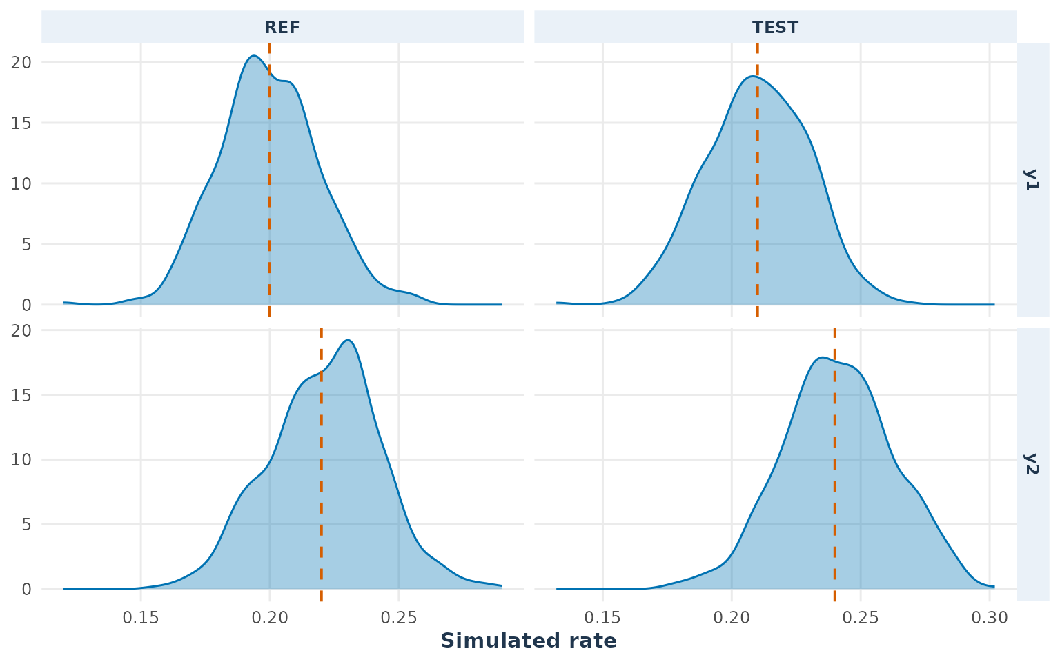

The empirical rate distributions should be centered near the values in count_rates.

3b. Endpoint correlations

plot_distribution(poisson_diagnostic, estimand = "correlation",
                  arms = c("TEST", "REF"))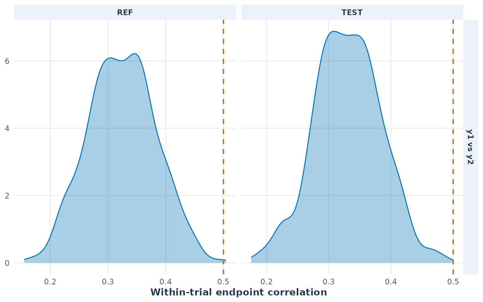

The dashed line is the latent correlation supplied through count_corr (Nelsen 2006). The observed Pearson correlation can differ because the latent normal variables are transformed into discrete counts. The plot checks the direction and approximate magnitude of the generated dependence; endpoint_corr is the exact parameter check.

3c. Estimand direction and sampling distribution

plot_distribution(poisson_diagnostic, estimand = "outcome", type = "histogram")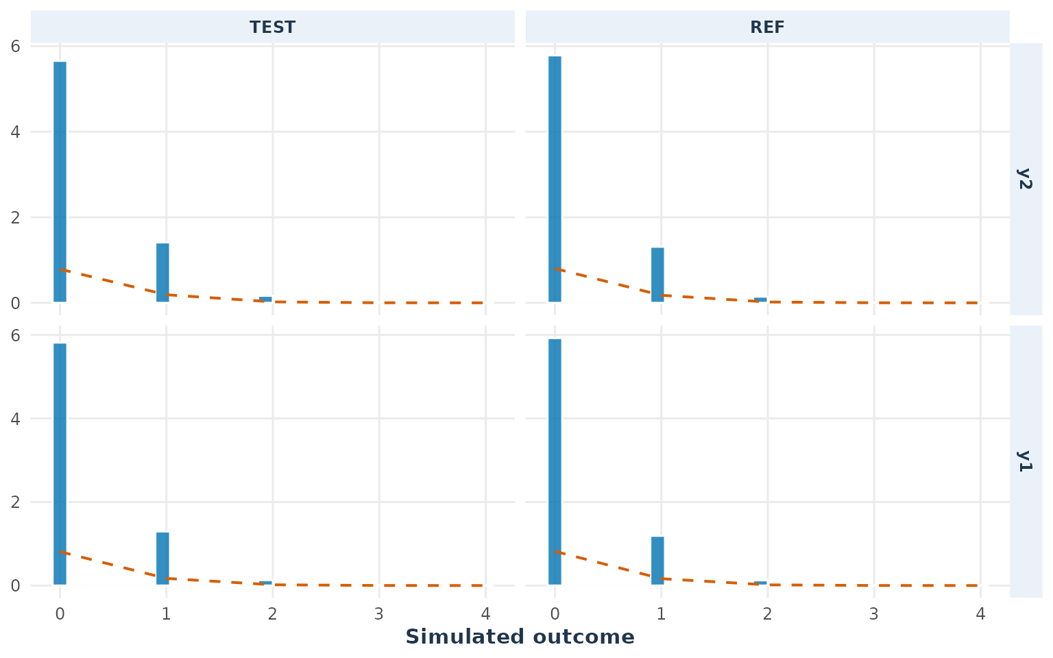

The empirical counts should be compatible with the Poisson reference distribution.

plot_distribution(poisson_diagnostic, estimand = "RR")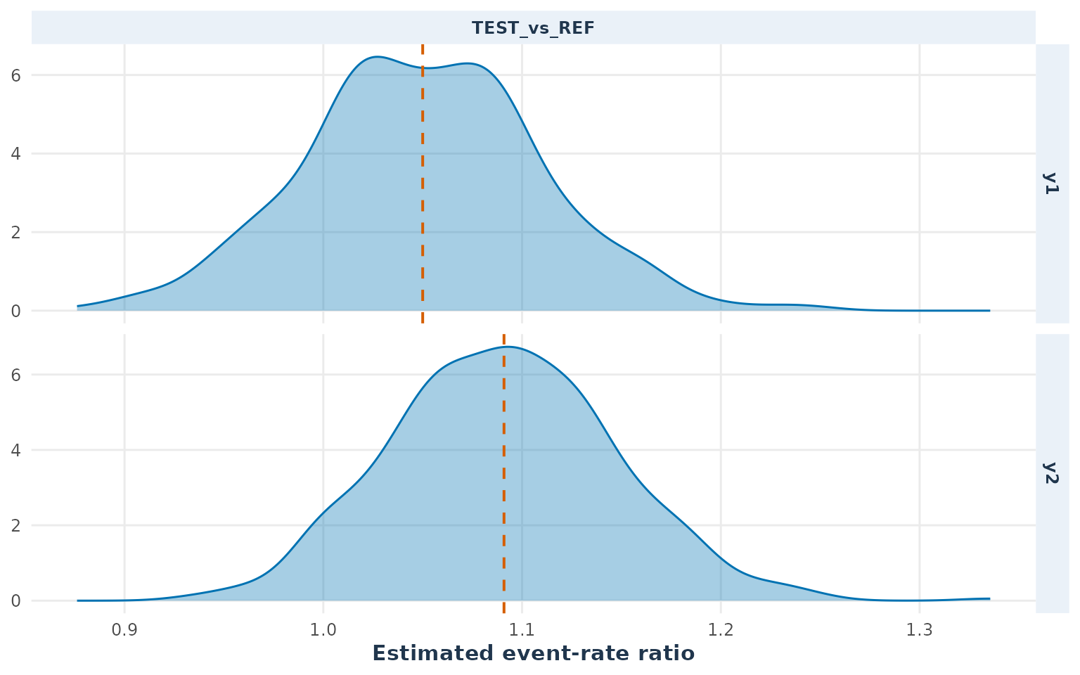

Step 4: Check Monte Carlo stability and precision

plot_stability(poisson_diagnostic)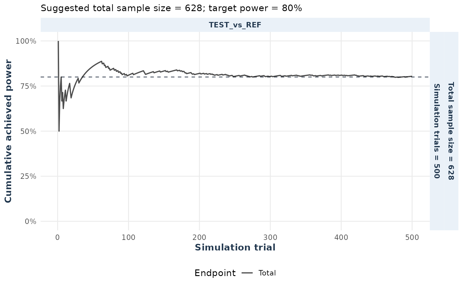

plot_mc_error(poisson_diagnostic)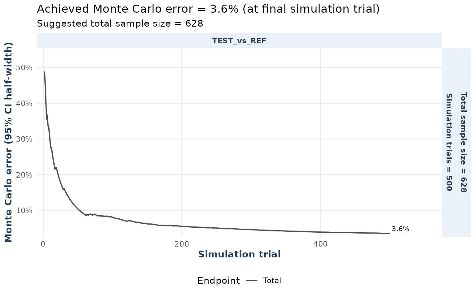

Step 5: Check Type I error at the equivalence boundaries

type1_one <- type1Error(x = poisson_diagnostic, null = "both", joint = TRUE)
plot(type1_one)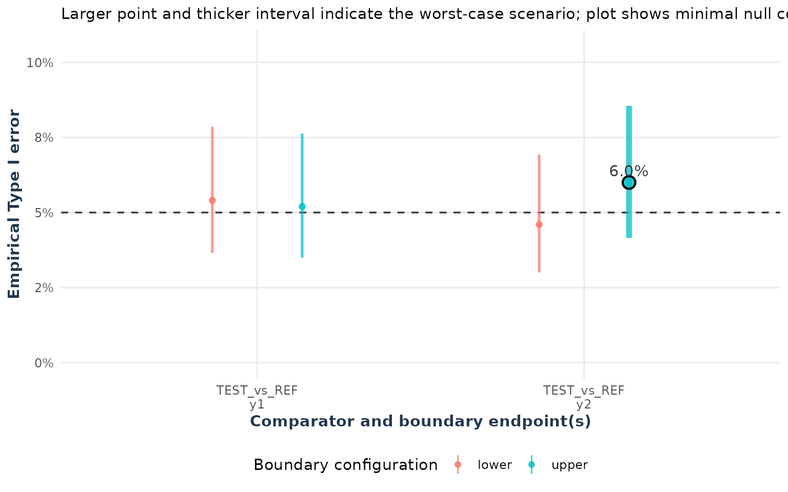

Step 6: Run the final sample-size calculation

This call uses exactly the rates, exposure, correlation matrix, margins, and parallel design used by poisson_diagnostic.

poisson_sample_size <- sampleSize(
  power = 0.80, distribution = "pois", rate_list = count_rates,
  list_comparator = count_comparators,
  list_lequi.tol = count_lower, list_uequi.tol = count_upper,
  exposure = count_exposure, cor_mat = count_corr, dtype = "parallel",
  lower = 100, upper = 1000, nsim = 1000, seed = 1234, ncores = 1,
  keep_sim_data = TRUE
)
summary(poisson_sample_size)
#> Sample Size Summary
#> ---------------------- 
#> Design type        : parallel 
#> Distribution       : pois 
#> Comparison type    : RR
#> Estimand           : event-rate ratio (lambda_T / lambda_R)
#> Hypotheses         : H0: RR <= L or >= U; H1: L < RR < U
#> Alpha              : 0.05 
#> Target power       : 0.8000 
#> Achieved power     : 0.8010 
#> Power interval     : [0.7746, 0.8250] 
#> Required endpoints : 2 
#> Alpha adjustment   : none 
#> 
#> Equivalence Margins:
#>   Comparison Endpoint Lower Upper
#>  TEST_vs_REF       y1   0.8  1.25
#>  TEST_vs_REF       y2   0.8  1.25
#> 
#> Estimated Sample Size:
#>  TEST REF Total
#>   316 316   632
confint(poisson_sample_size)
#>     Lower     Upper 
#> 0.7748841 0.8253299 
#> attr(,"conf.level")
#> [1] 0.95

For final planning, increase nsim and independently verify the selected sample size with simPower().

plot(poisson_sample_size)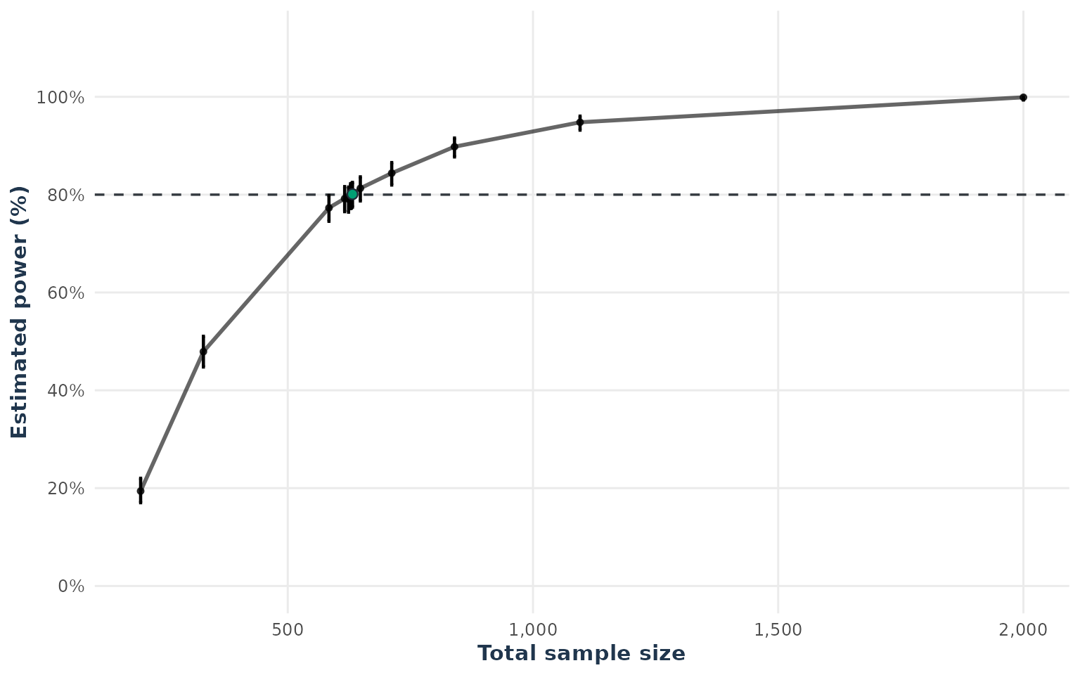

Repeat with a negative-binomial distribution

The negative-binomial calculation keeps the same rates, exposure, correlation, margins, and parallel design. The dispersion parameter allows the count variance to exceed its Poisson value. We use dispersion = 0.50 here as a deliberately visible sensitivity example. For a mean count near 2, the Poisson variance is about 2, whereas the negative-binomial variance is approximately 2 + 0.50 * 2^2 = 4.

nb_dispersion <- 0.50
negative_binomial_sample_size <- update(poisson_sample_size,
                                        distribution = "nbinom",
                                        dispersion = nb_dispersion)

summary(negative_binomial_sample_size)
#> Sample Size Summary
#> ---------------------- 
#> Design type        : parallel 
#> Distribution       : nbinom 
#> Comparison type    : RR
#> Estimand           : event-rate ratio (lambda_T / lambda_R)
#> Hypotheses         : H0: RR <= L or >= U; H1: L < RR < U
#> Alpha              : 0.05 
#> Target power       : 0.8000 
#> Achieved power     : 0.8000 
#> Power interval     : [0.7736, 0.8241] 
#> Required endpoints : 2 
#> Alpha adjustment   : none 
#> 
#> Equivalence Margins:
#>   Comparison Endpoint Lower Upper
#>  TEST_vs_REF       y1   0.8  1.25
#>  TEST_vs_REF       y2   0.8  1.25
#> 
#> Estimated Sample Size:
#>  TEST REF Total
#>   443 443   886
confint(negative_binomial_sample_size)
#>     Lower     Upper 
#> 0.7738406 0.8243794 
#> attr(,"conf.level")
#> [1] 0.95

plot_distribution(negative_binomial_sample_size, estimand = "outcome", type = "histogram")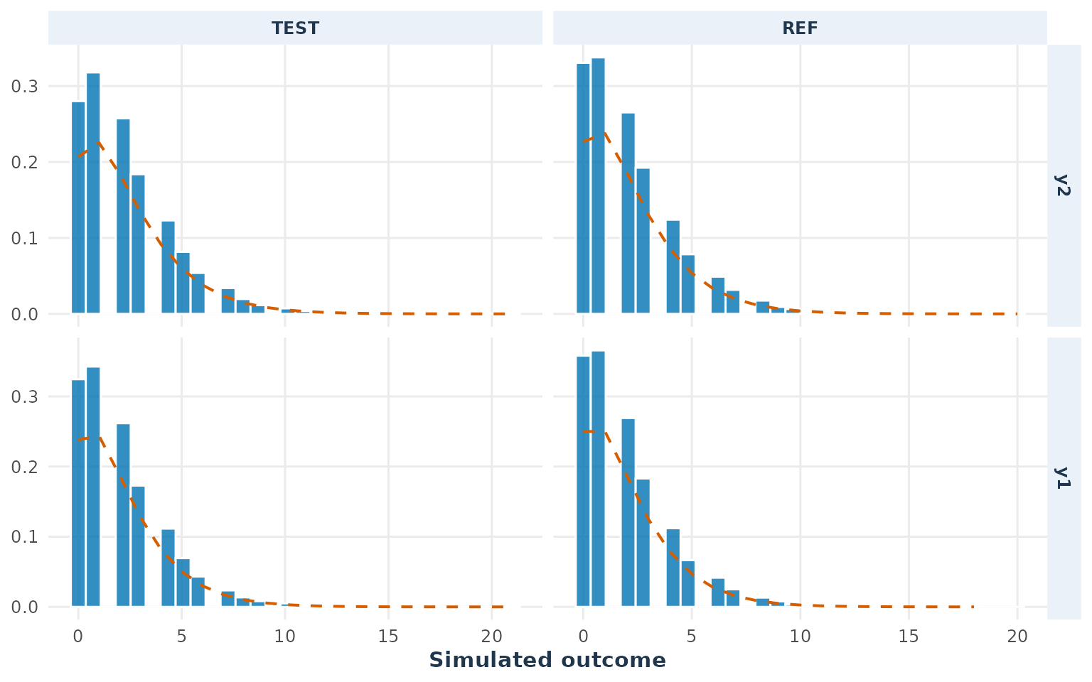

The result is conditional on nb_dispersion; vary it in sensitivity analyses when overdispersion is uncertain.

Use the same settings for a two-by-two crossover design

In a crossover design calculation, the count-model inputs from the parallel design are still needed: rate_list, exposure, dispersion (for a negative-binomial model), list_comparator, the equivalence margins, and the endpoint correlation. These describe the treatment effect and the count distribution. The crossover design additionally describes how each participant contributes observations under both treatments:

sigmaB is the between-participant standard deviation on the log-rate scale. It represents persistent participant-to-participant heterogeneity in event rates.
Eper is a length-two vector of period effects on the log-rate scale. For example, c(0, 0.10) means that the second period has a 0.10 log-rate increase relative to the first period.
Eco is a length-two vector of carry-over effects, ordered as reference carry-over and treatment carry-over. Use c(0, 0) when there is no carry-over effect assumed.
dropout is a length-two vector of dropout proportions for the two sequences. Use c(0, 0) when no dropout is expected.

For the crossover design, exposure refers to the observation time or opportunity for each treatment-period count. A participant contributes one count under each treatment when complete. For dtype = "2x2", n and n_per_arm refer to participants per sequence, not the total number of participants across both sequences. The crossover-specific parameters should be obtained from pilot data or subject-matter knowledge; they should not be copied from the parallel-arm standard deviations.


crossover_sample_size <- update(negative_binomial_sample_size,
                                dtype = "2x2",
                                sigmaB = 0.30,
                                Eper = c(0, 0.10),
                                Eco = c(0, 0),
                                dropout = c(0.10, 0.10))

summary(crossover_sample_size)
#> Sample Size Summary
#> ---------------------- 
#> Design type        : 2x2 
#> Distribution       : nbinom 
#> Comparison type    : RR
#> Estimand           : event-rate ratio (lambda_T / lambda_R)
#> Hypotheses         : H0: RR <= L or >= U; H1: L < RR < U
#> Alpha              : 0.05 
#> Target power       : 0.8000 
#> Achieved power     : 0.8160 
#> Power interval     : [0.7903, 0.8393] 
#> Required endpoints : 2 
#> Alpha adjustment   : none 
#> 
#> Equivalence Margins:
#>   Comparison Endpoint Lower Upper
#>  TEST_vs_REF       y1   0.8  1.25
#>  TEST_vs_REF       y2   0.8  1.25
#> 
#> Estimated Sample Size:
#>  seq0 seq1 Total
#>   232  232   514
confint(crossover_sample_size)
#>     Lower     Upper 
#> 0.7905659 0.8395577 
#> attr(,"conf.level")
#> [1] 0.95

The crossover design calculation uses the same treatment-effect and endpoint settings but evaluates paired treatment-period data. The values above are illustrative; in an actual study, sigmaB, period effects, carry-over effects, and sequence-specific dropout should be justified from prior data or a sensitivity analysis.

Chang, Yu-Wei, Yi Tsong, and Zhigen Zhao. 2017. “Sample Size Determination for a Three-Arm Equivalence Trial of Poisson and Negative Binomial Responses.” Journal of Biopharmaceutical Statistics 27 (2): 239–56. https://doi.org/10.1080/10543406.2016.1269787.

Nelsen, Roger B. 2006. An Introduction to Copulas. 2nd ed. Springer.

Zhu, Haiyuan. 2017. “Sample Size Calculation for Comparing Two Poisson or Negative Binomial Rates in Non-Inferiority or Equivalence Trials.” Statistics in Biopharmaceutical Research 9 (1): 107–15. https://doi.org/10.1080/19466315.2016.1225594.