

Estimate CATE scores for binary, count and survival outcomes. Binary scores include pooled logistic regression, doubly robust two-regression estimation and boosting. Count and survival methods include both outcome-regression and doubly robust scores. Continuous outcomes are not yet implemented.
Usage
catefit(
  response,
  data,
  score.method,
  cate.model,
  ps.model,
  ps.method = "glm",
  init.model = NULL,
  initial.predictor.method = NULL,
  ipcw.model = NULL,
  ipcw.method = "breslow",
  minPS = 0.01,
  maxPS = 0.99,
  followup.time = NULL,
  tau0 = NULL,
  higher.y = TRUE,
  prop.cutoff = seq(0.5, 1, length = 6),
  surv.min = 0.025,
  xvar.smooth.score = NULL,
  xvar.smooth.init = NULL,
  tree.depth = 2,
  n.trees.rf = 1000,
  n.trees.boosting = 200,
  B = 3,
  Kfold = 5,
  error.maxNR = 0.001,
  max.iterNR = 150,
  tune = c(0.5, 2),
  seed = NULL,
  plot.gbmperf = TRUE,
  verbose = 0,
  contrast.control = list(),
  rmst.control = list(),
  ps.control = list(),
  rf.control = list(),
  ...
)
Arguments
- response
A string describing the type of outcome in the data. Allowed values include "binary", "count" (see
catecvcount()), "survival" (seecatecvsurv()) and "continuous" (seecatecvmean()).- data
A data frame containing the variables in the outcome, treatment, and censoring models (if specified); a data frame with
nrows (1 row per observation).- score.method
A vector of one or multiple methods to estimate the CATE score. Allowed values are:
'boosting','twoReg','contrastReg','poisson'(count and survival outcomes only),'randomForest'(survival, continuous outcomes only),negBin(count outcomes only),'gam'(continuous outcomes only),'gaussian'(continuous outcomes only). For binary outcomes, use'logistic','twoReg', or'boosting'.- cate.model
A formula describing the outcome model to be fitted. The outcome must appear on the left-hand side. For survival outcomes, a
Survobject must be used to describe the outcome.- ps.model
A formula describing the treatment model (propensity-score model) to be fitted. The treatment must appear on the left-hand side. For binary outcomes, logical treatment values
FALSEandTRUEare mapped to 0 and 1, respectively. Numeric 0/1 values or two distinct treatment labels are also accepted. If data are from a randomized controlled trial, specifyps.model = trt ~ 1as an intercept-only model.- ps.method
A character value for the method to estimate the propensity score. Allowed values include one of:
'glm'for logistic regression with main effects only (default), or'lasso'for a logistic regression with main effects and LASSO penalization on two-way interactions (added to the model if interactions are not specified inps.model). Relevant only whenps.modelhas more than one variable.- init.model
A formula describing the initial predictor model. The outcome must appear on the left-hand side. It must be specified when
score.method = contrastRegortwoReg, except for binary outcomes, which usecate.model.- initial.predictor.method
A character vector for the method used to get initial outcome predictions conditional on the covariates specified in
cate.model. Only applies whenscore.methodincludes'twoReg'or'contrastReg'.Allowed values include one of'randomForest'(survival outcomes only),'boosting','logistic'(survival outcomes only, fast),'poisson'(count outcomes only, fast),'gaussian'(continuous outcomes only) and'gam'(count and continuous outcomes only). Default isNULL, which assigns'boosting'for count outcomes and'randomForest'for survival outcomes.- ipcw.model
A formula describing the censoring model used for inverse probability of censoring weighting (IPCW). The left-hand side must be empty. Only applies for survival outcomes. Default is
NULL, which uses a censoring model with the same covariates as the outcome modelcate.model, plus the treatment.- ipcw.method
A character value for the censoring model. Only applies for survival outcomes. Allowed values are:
'breslow'(Cox regression with Breslow estimator of t he baseline survivor function),'aft (exponential)','aft (weibull)','aft (lognormal)'or'aft (loglogistic)'(accelerated failure time model with different distributions for y variable). Default is'breslow'.- minPS
A numerical value (in `[0, 1]`) below which estimated propensity scores should be truncated. Default is
0.01.- maxPS
A numerical value (in `(0, 1]`) above which estimated propensity scores should be truncated. Must be strictly greater than
minPS. Default is0.99.- followup.time
A column name in
dataspecifying the maximum follow-up time, interpreted as the potential censoring time. Only applies for survival outcomes. Default isNULL, which corresponds to unknown potential censoring time.- tau0
The truncation time for defining restricted mean time lost. Only applies for survival outcomes. Default is
NULL, which corresponds to setting the truncation time as the maximum survival time in the data.- higher.y
A logical value indicating whether higher (
TRUE) or lower (FALSE) values of the outcome are more desirable. Default isTRUE.- prop.cutoff
A vector of numerical values (in `(0, 1]`) specifying percentiles of the estimated log CATE scores to define nested subgroups. Each element represents the cutoff to separate observations in nested subgroups (below vs above cutoff). The length of
prop.cutoffis the number of nested subgroups. An equally-spaced sequence of proportions ending with 1 is recommended. Default isseq(0.5, 1, length = 6).- surv.min
Lower truncation limit for the probability of being censored. It must be a positive value and should be chosen close to 0. Only applies for survival outcomes. Default is
0.025.- xvar.smooth.score
A vector of characters indicating the name of the variables used as the smooth terms if
score.method = 'gam'. The variables must be selected from the variables listed incate.model.- xvar.smooth.init
A vector of characters indicating the name of the variables used as the smooth terms if
initial.predictor.method = 'gam'. The variables must be selected from the variables listed ininit.model. Default isNULL, which uses all variables ininit.model.- tree.depth
A positive integer specifying the depth of individual trees in boosting (usually 2-3). Used only if
score.method = 'boosting'or ifinitial.predictor.method = 'boosting'withscore.method = 'twoReg'or'contrastReg'. Default is 2.- n.trees.rf
A positive integer specifying the number of trees in random forest. Used if
score.method = 'randomForest'or ifinitial.predictor.method = 'randomForest'withscore.method = 'twoReg'or'contrastReg'. Only applies for survival outcomes. Default is1000.- n.trees.boosting
A positive integer specifying the maximum number of trees in boosting (usually 100-1000). Used if
score.method = 'boosting'or ifinitial.predictor.method = 'boosting'withscore.method = 'twoReg'or'contrastReg'. Default is200.- B
A positive integer specifying the number of time cross-fitting is repeated in
score.method = 'twoReg'and'contrastReg'. Default is3.- Kfold
A positive integer specifying the number of folds used in cross-fitting to partition the data in
score.method = 'twoReg'and'contrastReg'. Default is5.- error.maxNR
A numerical value > 0 indicating the minimum value of the mean absolute error in Newton Raphson algorithm. Used only if
score.method = 'contrastReg'. Default is0.001.- max.iterNR
A positive integer indicating the maximum number of iterations in the Newton Raphson algorithm. Used only if
score.method = 'contrastReg'. Default is150.- tune
A vector of 2 numerical values > 0 specifying tuning parameters for the Newton Raphson algorithm.
tune[1]is the step size,tune[2]specifies a quantity to be added to diagonal of the slope matrix to prevent singularity. Used only ifscore.method = 'contrastReg'. Default isc(0.5, 2).- seed
An optional integer specifying an initial randomization seed for reproducibility. Default is
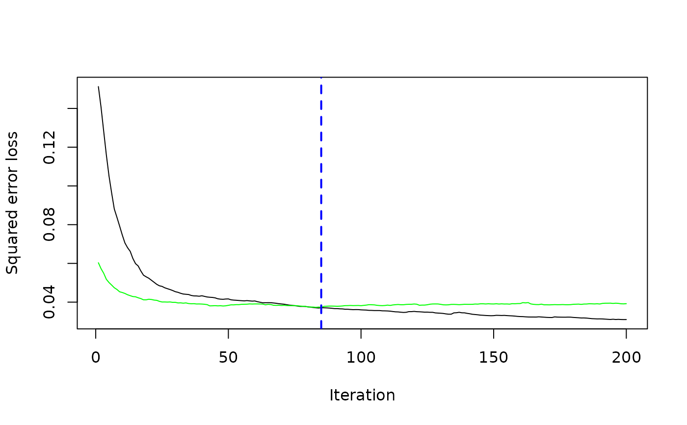
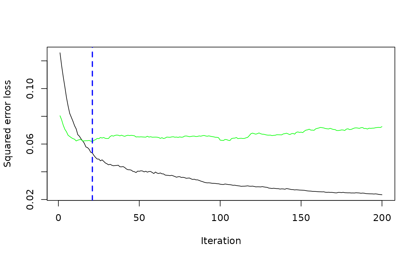
NULL, corresponding to no seed.- plot.gbmperf
A logical value indicating whether to plot the performance measures in boosting. Used only if
score.method = 'boosting'or ifscore.method = 'twoReg'or'contrastReg'andinitial.predictor.method = 'boosting'. Default isTRUE.- verbose
An integer value indicating whether intermediate progress messages and histograms should be printed.
1indicates messages are printed and0otherwise. Default is0.- contrast.control
A named list of options for count or survival contrast regression. Supported names are
solver("C", the default, or"R"),error.maxNR,max.iterNR,tune, andoptim.control(a named list passed tostats::optimon fallback). List entries override the corresponding top-level NR arguments. Options are kept separate from..., which is forwarded to boosting. Count and survival outcomes support this list; continuous outcomes retain their existing solver.- rmst.control
Named options for Cox restricted mean survival integration. Supported entry:
solver = "C"(default) orsolver = "R". The C backend accumulates each patient's integral without allocating a patient-by-event-time matrix. Cox model fitting is unchanged. Available only for survival outcomes; independent ofcontrast.control.- ps.control
Named options for LASSO propensity-score interaction screening. Supported entry:
solver = "C"(default) orsolver = "R". Only affects screening whenps.method = "lasso"; the LASSO fit and interaction selection rule are unchanged. Kept separate from boosting's...and other numerical controls.- rf.control
Named list of randomForestSRC options:
mtry,nodesize,nsplit,nodedepth, andsplitrule. Applies to both treatment arms and survival initial-predictor forests. Usen.trees.rffor the number of trees.- ...
Additional boosting arguments; see
boosting-control.For
response = "binary",score.method = "logistic"fits a logistic model with treatment interactions."twoReg"cross-fits separate logistic outcome models and a treatment model, then projects the augmented inverse-propensity outcomes for each arm onto the covariates incate.modelusing linear regression. The score is the difference of these projections, averaged overBrepetitions ofKfoldfolds. It estimates the linear projection of the conditional risk difference if either the treatment model or both outcome models are correct, under identification and positivity assumptions. Propensity score truncation can affect this property. The projection need not lie between -1 and 1 and equals the conditional risk difference only if that difference is linear in the specified design. The difference between arm coefficients is returned incoefficients$twoRegand bycoef(); the separate arm coefficients are stored infit$twoReg$coefficients. Logistic model coefficients are on the log-odds scale and are stored infit$logistic; they are not linear risk-difference score coefficients. Boosting does not have a linear score coefficient vector. With neithertwoRegnor another linear binary score,coef()returnsNULL."boosting"fits separate Bernoulli gradient-boosting models in each treatment arm, with the number of trees selected by five-fold cross-validation. All three scores are predicted risk differences; subgroup effects are doubly robust risk differences. Binary boosting requires at least one outcome-model covariate and both outcome values in each arm. Its fitted models and selected tree counts are stored infit$boosting. Scores and subgroup effects are estimated on the same data; they are not independent validation. For extra boosting controls, seeboosting-control. Subgroup fits without both arms or with rank-deficient models return NA.
Value
Fitted objects retain treatment.labels in treatment 0/1 order
for score plot labels. For count response, see description of other outputs in catefitcount().
For survival response, see description of outputs in catefitsurv().
Details
For count response, see details in catefitcount().
For survival response, see details in catefitsurv().
References
Yadlowsky, S., Pellegrini, F., Lionetto, F., Braune, S., & Tian, L. (2020). Estimation and validation of ratio-based conditional average treatment effects using observational data. Journal of the American Statistical Association, 1-18. DOI: 10.1080/01621459.2020.1772080.
Hoogland, J., Debray, T. P. A., Desachy, G., & Nguyen, T.-L. (2026). Introduction to methods for personalizing medicine. In T. P. A. Debray, T.-L. Nguyen, & R. W. Platt (Eds.), Comparative Effectiveness and Personalized Medicine Research Using Real-World Data (Chapter 17, pp. 421–463). Chapman & Hall/CRC. doi:10.1201/9781003300809-17
Hoogland, J., IntHout, J., Belias, M., et al. (2021). A tutorial on individualized treatment effect prediction from randomized trials with a binary endpoint. Statistics in Medicine, 40(26), 5961–5981. doi:10.1002/sim.9154
Jiang, X., Simoneau, G., Pellegrini, F., Shen, C., de Moor, C., & Tian, L. (2026). Visualization and interpretation of individualized treatment rule results. In T. P. A. Debray, T.-L. Nguyen, & R. W. Platt (Eds.), Comparative Effectiveness and Personalized Medicine Research Using Real-World Data (Chapter 20, pp. 513–536). Chapman & Hall/CRC. doi:10.1201/9781003300809-20
Examples
# Count outcome
fit_1 <- catefit(response = "count",
data = countExample,
score.method = "poisson",
cate.model = y ~ age + female + previous_treatment +
previous_cost + previous_number_relapses +
offset(log(years)),
ps.model = trt ~ age + previous_treatment,
higher.y = TRUE,
seed = 999)
#> Variable trt was recoded to 0/1 with drug0->0 and drug1->1.
coef(fit_1)
#> poisson
#> (Intercept) -0.58185218
#> age -0.01117701
#> female 0.58829733
#> previous_treatmentdrugB 0.73724361
#> previous_treatmentdrugC 0.15545985
#> previous_cost -0.13035642
#> previous_number_relapses -0.05339112
# \donttest{
# Survival outcome
library(survival)
tau0 <- with(survivalExample,
min(quantile(y[trt == "drug1"], 0.95), quantile(y[trt == "drug0"], 0.95)))
fit_2 <- catefit(response = "survival",
data = survivalExample,
score.method = c("poisson", "boosting", "randomForest"),
cate.model = Surv(y, d) ~ age + female + previous_cost +
previous_number_relapses,
ps.model = trt ~ age + previous_treatment,
initial.predictor.method = "logistic",
ipcw.model = ~ age + previous_cost + previous_treatment,
tau0 = tau0, higher.y = TRUE, seed = 999, n.cores = 1)
#> Variable trt was recoded to 0/1 with drug0->0 and drug1->1.
 #> Warning: Warning(s) occurred when estimating the ATEs in the nested subgroup using "poisson"
#> Warning: Warning: Warning(s) occurred when estimating the ATEs in the nested subgroup using "poisson"; see 'errors/warnings'.
coef(fit_2)
#> poisson
#> (Intercept) 0.46109243
#> age -0.24335209
#> female 0.12532711
#> previous_cost 0.89803249
#> previous_number_relapses -0.02470863
# }