precmed: Precision Medicine in R

A doubly robust precision medicine approach to estimate and validate conditional average treatment effects

Examples with survival outcome of the entire workflow

Load required packages

library(precmed)
library(dplyr)
library(ggplot2)

Load data set (Example data with survival outcome)

To show the functionalities of the precmed package for survival outcomes we first need data. For our examples we use simulated data that is located in the survivalExample data set. The data set survivalExample was simulated based on real-world claims data in multiple sclerosis and has 4,000 observations and 9 variables.

	level	Overall	drug0	drug1
Number of patients		4000	1849	2151
Age (mean (SD))		45.8 (9.9)	37.3 (6.4)	53.1 (5.5)
Gender (%)	male	996 (24.9)	456 (24.7)	540 (25.1)
	female	3004 (75.1)	1393 (75.3)	1611 (74.9)
Previous treatment (%)	drugA	1752 (43.8)	819 (44.3)	933 (43.4)
	drugB	459 (11.5)	207 (11.2)	252 (11.7)
	drugC	1789 (44.7)	823 (44.5)	966 (44.9)
Previous medical cost ($) (mean (SD))		14362.0 (24265.9)	11358.0 (14393.2)	16944.1 (30045.6)
Previous number of symptoms (%)	0	347 ( 8.7)	191 (10.3)	156 ( 7.3)
	1	2686 (67.2)	1219 (65.9)	1467 (68.2)
	>=2	967 (24.2)	439 (23.7)	528 (24.5)
Previous number of relapses (%)	0	2612 (65.3)	1247 (67.4)	1365 (63.5)
	1	1106 (27.7)	488 (26.4)	618 (28.7)
	2	246 ( 6.2)	99 ( 5.4)	147 ( 6.8)
	3	33 ( 0.8)	14 ( 0.8)	19 ( 0.9)
	4	2 ( 0.0)	1 ( 0.1)	1 ( 0.0)
	5	1 ( 0.0)	0 ( 0.0)	1 ( 0.0)
Days until the first relapse (mean(SD))		141.6 (262.2)	152.6 (275.5)	132.1 (249.9)
Event indicator (0: censoring, 1: relapse) (%)	0	3352 (83.8)	1695 (91.7)	1657 (77.0)
	1	648 (16.2)	154 ( 8.3)	494 (23.0)

Most variables are baseline patient characteristics like age, gender, and previous treatment.

We will use y as the survival outcome, which is the number of days until the first relapse or censoring, whichever comes first.
We will use d as the event indicator, where $1$ represents an event and $0$ represents censoring. The censoring rate is about 84%.
We will use trt as the treatment variable, which has 2 drugs (drug0 and drug1).

To avoid multicollinearity issues, the continuous variable age was centered at 48 years old and the medical costs in the year prior to treatment initiation previous_cost was centered at 14,362 USD and scaled with standard deviation 24,266 USD.

The final dataset survivalExample looked like this:

#> 'data.frame':    4000 obs. of  9 variables:
#>  $ age                     : num [1:4000, 1] -26.83 -2.83 -12.83 -20.83 6.17 ...
#>   ..- attr(*, "scaled:center")= num 45.8
#>  $ female                  : int  1 1 1 0 0 1 1 1 1 1 ...
#>  $ previous_treatment      : Factor w/ 3 levels "drugA","drugB",..: 3 1 3 1 3 1 3 3 3 1 ...
#>  $ previous_cost           : num [1:4000, 1] -0.341 -0.239 -0.171 -0.392 -0.518 ...
#>   ..- attr(*, "scaled:center")= num 14362
#>   ..- attr(*, "scaled:scale")= num 24266
#>  $ previous_number_symptoms: Factor w/ 3 levels "0","1",">=2": 2 2 2 3 3 2 3 2 2 2 ...
#>  $ previous_number_relapses: int  0 1 2 0 1 0 0 2 0 0 ...
#>  $ trt                     : Factor w/ 2 levels "drug0","drug1": 1 1 1 1 2 1 2 2 2 2 ...
#>  $ y                       : num  102.1 51.3 104.9 61.5 35.6 ...
#>  $ d                       : num  0 0 0 0 0 0 0 0 0 1 ...

Estimation of the ATE with `atefit()`

First, one might be interested in the effect of the drug (trt) on the number of days until the first relapse or censoring (y). Lets test this using Cox regression.

library(survival)
output_cox <- coxph(Surv(y, d) ~ trt, data = survivalExample)
summary(output_cox)
#> Call:
#> coxph(formula = Surv(y, d) ~ trt, data = survivalExample)
#> 
#>   n= 4000, number of events= 648 
#> 
#>             coef exp(coef) se(coef)     z Pr(>|z|)    
#> trtdrug1 1.11311   3.04381  0.09233 12.06   <2e-16 ***
#> ---
#> Signif. codes:  0 '***' 0.001 '**' 0.01 '*' 0.05 '.' 0.1 ' ' 1
#> 
#>          exp(coef) exp(-coef) lower .95 upper .95
#> trtdrug1     3.044     0.3285      2.54     3.648
#> 
#> Concordance= 0.639  (se = 0.009 )
#> Likelihood ratio test= 170.1  on 1 df,   p=<2e-16
#> Wald test            = 145.3  on 1 df,   p=<2e-16
#> Score (logrank) test = 160.9  on 1 df,   p=<2e-16

We see from the Cox regression we see that drug1 resulted in a hazard ratio (HR) of 3.04 when compared to drug 0. This indicates that drug 0 is superior to drug 1 because drug 1 increases the risk of a relapse.

Now we want to estimate the Average Treatment Effect (ATE) and correct for several covariates like age and previous treatment because they might influence the relation between treatment and outcome. The atefit() function allows estimating the ATE in terms of restricted mean time lost (RMTL) and HR (hazard ratio). The RMTL estimator is doubly robust, meaning that the estimator is consistent if the PS model (argument ps.model) or the outcome model (argument cate.model) or both are correctly specified. The estimator also depends on the estimation of Inverse Probability Censoring Weights (IPCW). The HR estimator is based on a Cox regression model. The function also provides standard error, confidence intervals, and p-values based on bootstrap.

The mandatory arguments for atefit() are:

The response argument specifies the type of outcome in the data. For survival outcomes, response = “survival”. This informs the function of the necessary arguments and methods to use.
The argument data indicates the data frame in which the outcome, treatment and covariates specified in either cate.model or ps.model should be fetched.
The score.method argument specifies the precision medicine (PM) methods to be used to calculate the CATE scores. There are a total of 5 scoring methods implemented:
- poisson fits a Poisson model separately by treatment group.
- boosting uses gradient boosted regression models (GBM) separately by treatment group.
- randomForest fits a random forest model by treatment group.
- twoReg implements the doubly robust two regressions estimator in @yadlowsky2020estimation.
- contrastReg implements the doubly robust contrast regression estimator from @yadlowsky2020estimation.
The argument cate.model specifies the CATE model as a formula, with the survival object from the survival package, Surv(y, d), supplied on the left-hand side and the explanatory covariates supplied on the right-hand side. In the example below, we chose to specify to CATE as a linear combination of the following covariates: age, sex, medical costs in the year prior to treatment initiation, and number of relapses in the year prior to treatment initiation. Non-linear or interaction terms could also be included. Note that the treatment variable is not supplied in cate.model since this is an outcome model.
The ps.model argument specifies the PS model as a formula, with the treatment variable trt on the left-hand side and the covariates (age and previous treatment in this example) on the right-hand side. The variable trt must be supplied as a numeric variable taking only 2 values, “1” for active treatment and “0” for control or comparator. If it is not the case, catecv() will stop with error if trt takes more than 2 distinct values or will automatically transform trt into a numeric variable. In this example, trt (a factor variable taking values “drug0” and “drug1”) was transformed and a warning message was left to the user (see output below): Variable trt was recoded to 0/1 with drug0->0 and drug1->1. If the data are from a RCT, it suffices to specify ps.model = trt ~ 1. Note that the PS model is only used in the estimation of the 2 doubly robust methods (two and contrast regressions).
tau0: The truncation time for defining restricted mean time lost. Because our outcome y is skewed towards 0, we use the 95% upper limit.

Let’s calculate the ATE for the effect of treatment on y and build an outcome model that contains all variables and a PS model with age and previous_treatment.

#define tau0
tau0 <- with(survivalExample,
             min(quantile(y[trt == "drug1"], 0.95), quantile(y[trt == "drug0"], 0.95)))

#run atefit
output_atefit <- atefit(response = "survival",
                        data = survivalExample,
                        cate.model = survival::Surv(y, d) ~ age + female + previous_cost + previous_number_relapses,
                        ps.model = trt ~ age + previous_treatment,
                        tau0 = tau0)
#> Warning in data.preproc.surv(fun = "drinf", cate.model = cate.model, ps.model = ps.model, : Variable trt was recoded to 0/1 with drug0->0 and drug1->1.

When verbose = 1, the function outputs a progress bar in the console.

output_atefit
#> Average treatment effect:
#> 
#>                   estimate         SE    CI.lower  CI.upper     pvalue
#> log.rmtl.ratio   0.0701553 0.03457152 0.002396377 0.1379142 0.04242973
#> log.hazard.ratio 2.7133243 0.20509341 2.311348600 3.1153000 0.00000000
#> 
#> Estimated RMST:
#> 
#>       estimate       SE CI.lower CI.upper pvalue
#> rmst1 172.8609 6.171134 160.7657 184.9561      0
#> rmst0 196.5603 8.837641 179.2388 213.8817      0
#> Warning in print.atefit(x): Variable trt was recoded to 0/1 with drug0->0 and drug1->1.

The output of atefit() shows the point estimate, standard error (“SE”), lower (“CI.lower”) and upper (“CI.upper”) bound of the 95% confidence interval, and the p-value (“pvalue”) for 4 estimands:

the restricted mean survival time under drug 1 ($rmst1)
the restricted mean survival time under drug 0 ($rmst0)
the log RMTL ratio ($log.rmtl.ratio), which is the log of the ratio of tau0 - $rmst1 divided by tau0 - $rmst0
the log HR ($log.hazard.ratio).

For example, the log RMTL ratio of 0.07 and the 95% confidence interval of (0, 0.14) are displayed in the output. The RMTL ratio of along with the 95% confidence interval suggest that drug 0 is superior to drug 1 because the ratio is significantly greater than 1. When we check the estimated RMST, we also see that the estimated rmst1 is lower compared to rmst0, indicating that patients that received drug0 have a longer mean survival time compared to drug1.

The output of atefit() is expressed in terms of treatment 0 vs 1, where the RMTL and hazard ratios are expressed as the ratio of the treatment coded as 1 over the treatment coded as 0. If the treatment variable is not coded as 0/1 in the data set, the function returns a warning output_atefit$warning which indicates what key was used to recode the treatment variable into a 0/1 variable.

output_atefit$warning
#> [1] "Variable trt was recoded to 0/1 with drug0->0 and drug1->1.\n"

Using plot(output_atefit), a histograms is generated of the point estimates across the n.boot bootstrap iterations for 4 estimands (rmst1, rmst0, log.rmtl.ratio, log.hazard.ratio). A red vertical line is added to each histogram with the mean of the bootstrap estimates.

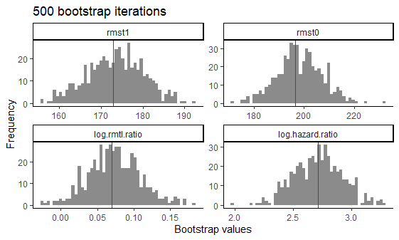
Histograms of bootstrap estimators for 4 estimands after 500 bootstrap

Estimation of the CATE score with `catefit()`

Now we have calculated the ATE we know the effect of both treatments on average, but this effect might not be the same for all patients. Thus, it might be worthwhile to check if there are subgroups that respond differently to the treatments. We can calculate the Conditional Average Treatment Effect (CATE) score which calculates the ATE for different subgroups in the data. If no internal validation is needed (we get back to that later), we can use the catefit() function to a model directly to the entire data set to estimate the CATE score. For the catefit() function we have to define the score.method. This arguments specifies the precision medicine (PM) method to be used to calculate the CATE scores. There are a total of 5 scoring methods implemented:

The mandatory arguments in catefit() are:

response: “survival” in this example because we use have data with a survival outcome (e.g., number of days until the first relapse or censoring))
data: the name of the data set. (survivalExample)
score.method: argument specifies the precision medicine (PM) methods to be used to calculate the CATE scores. There are a total of 5 scoring methods implemented:
- poisson fits a Poisson model separately by treatment group.
- boosting uses gradient boosted regression models (GBM) separately by treatment group.
- randomForest fits a random forest model by treatment group.
- twoReg implements the doubly robust two regressions estimator in @yadlowsky2020estimation.
- contrastReg implements the doubly robust contrast regression estimator from @yadlowsky2020estimation.
cate.model: A formula describing the outcome model to be fitted. The outcome must appear on the left-hand side. In the example, we choose to specify to outcome model as a linear combination of the following covariates: age, sex, medical costs in the year prior to treatment initiation, and number of relapses in the year prior to treatment initiation. Non-linear or interaction terms could also be included. Note that the treatment variable is not supplied in cate.model since this is an outcome model.
ps.model: A formula describing the propensity score (PS) model to be fitted. The treatment must appear on the left-hand side and the covariates (age and previous treatment in this example) on the right-hand side. The variable trt must be supplied as a numeric variable taking only 2 values, 1 for active treatment and 0 for control or comparator. If it is not the case, the function will stop with error if trt takes more than 2 distinct values or will automatically transform trt into a numeric variable. In this example, trt (a factor variable taking values “drug0” and “drug1”) was transformed and a warning message was left to the user (see output below): Variable trt was recoded to 0/1 with drug0->0 and drug1->1. If the data are from a RCT, it suffices to specify ps.model = trt ~ 1. Note that the PS model is only used in the estimation of the 2 doubly robust methods (two and contrast regressions).

We also specified the following non-mandatory arguments to fit with the data and problem at hand: initial.predictor.method, tau0, higher.y, seed, and plot.gbmperf.

initial.predictor.method specifies how predictions of the outcome are estimated in two regressions and contrast regression. Flexible models can be used such as GBM (“boosting”), random forests (“randomForest”) or logistic regression (“logistic”). We chose “logistic” because it is relatively faster than boosting methods and random forest.
tau0 is the truncation time for defining restricted mean time lost (RMTL). Because our outcome y is skewed towards 0, we use the 95% upper limit.
higher.y was set to TRUE because relapse is a negative event and longer time to first relapse is more desirable in our example. Hence, we are telling the function that subgroups of high responders to drug1 vs drug0 should have later onset of the first relapse. In other situation, higher outcomes may be more favorable for time to a positive event, e.g., time to discharge or time to improved disability. It is important for this argument to match with the nature of y outcome because it will affect how the subgroups are defined by the CATE scores and the performance metrics.
We set a random seed seed = 999 to reproduce the results.
We avoided generating the boosting performance plots by specifying plot.gbmperf = FALSE.

Please see the Function description section for details.

If you run into errors or warnings with your data, it might be helpful to go over the descriptions to see if you need to alter the default values. In this toy example, we keep the default values of the remaining arguments. For this toy example we selected randomForest and contrastReg to limit run time.

tau0 <- with(survivalExample,
             min(quantile(y[trt == "drug1"], 0.95), quantile(y[trt == "drug0"], 0.95)))

output_catefit <- catefit(response = "survival",
                          data = survivalExample,
                          score.method = c( "randomForest", "contrastReg"),
                          cate.model = survival::Surv(y, d) ~ age + female + previous_cost + previous_number_relapses,
                          ps.model = trt ~ age + previous_treatment,
                          initial.predictor.method = "logistic",
                          tau0 = tau0, 
                          higher.y = TRUE,
                          seed = 999,
                          plot.gbmperf = FALSE)
#> Warning in data.preproc.surv(fun = "catefit", cate.model = cate.model, ps.model = ps.model, : Variable trt was recoded to 0/1 with drug0->0 and drug1->1.

Each method specified in score.method has the following sets of results in catefit():

score contains the log-transformed estimated CATE scores for each subject. The CATE score is a linear combination of the variables specified in the cate.model argument. Same as the outcome, lower CATE scores are more desirable if higher.y = FALSE and vice versa. In our example, the survival outcome is time to first relapse, which is a negative event, so higher values indicate later onset of the first relapse. Hence, we specify higher.y = TRUE in the example. Each subject has 1 CATE score so the length of this output is 4,000 for our toy example. Below we show the CATE scores estimated with contrast regression for the first 6 subjects in the data.

length(output_catefit$score.contrastReg)
#> [1] 4000
head(output_catefit$score.contrastReg)
#> [1]  5.3264861  1.1651265  3.4845913  4.0150879 -0.8484891  2.4213491

coefficients contains the estimated coefficients of the CATE score for each scoring method. It is a data frame of the covariates (including intercept) as rows and scoring methods as columns. In our toy example, there are 4 covariates in the cate.model, plus the intercept, so there are 5 rows of estimated coefficients within each column. Boosting method does not estimate coefficients (it directly predicts the score) so they do not have coefficient results here.

output_catefit$coefficients
#>                          contrastReg
#> (Intercept)                0.2528396
#> age                       -0.1911735
#> female                     0.1359737
#> previous_cost              0.5634907
#> previous_number_relapses   0.3693452

We can define the estimated CATE scores for contrast regression like shown below. The user can use this information to study the influence of each covariate. $\begin{aligned} \widehat{CATE} = 0.25 & - 0.19 \times \text{age} \\ & + 0.14 \times \text{female (vs male)} \\ & + 0.56 \times \text{previous medical costs} \\ & + 0.37 \times \text{previous number of relapses} \end{aligned}$

ate contains estimated ATEs by each nested subgroup of high responders to drug 1 defined by prop.cutoff. The subgroups are defined based on the estimated CATE scores with the specified scoring method. In this example, we show the estimated ATEs of subgroups identified by CATE scores of the contrast regression. For example, the estimated ATE for the subgroup of subjects constructed based on the 50% (“prop0.5”) lowest CATE scores estimated from the contrast regression is 0.41.

output_catefit$ate.contrastReg
#>   prop0.5   prop0.6   prop0.7   prop0.8   prop0.9     prop1 
#> 0.4098373 0.5114925 0.6269751 0.7801699 0.9145661 1.0726748

You are encouraged to summarize and visualize the outputs in whichever way that fits their particular situation outside the package’s functions. For example, it is possible to plot the densities of all CATE scores with ggplot. There are some subjects with extremely high estimated CATE scores but most of the samples fall between -10 and 10.

dataplot <- data.frame(score = factor(rep(c("Random Forest", "Contrast regression"), 
                                          each = length(output_catefit$score.randomForest))), 
                       value = c(output_catefit$score.randomForest,output_catefit$score.contrastReg))

dataplot %>% 
  ggplot(aes(x = value, fill = score)) + 
  geom_density(alpha = 0.5) +
  theme_classic() + 
  labs(x = "Estimated CATE score", y = "Density", fill = "Method")
#> Warning: Removed 5 rows containing non-finite outside the scale range
#> (`stat_density()`).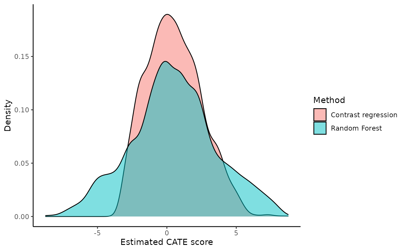

Internal validation via `catecv()`

The catecv() function provides the same estimation as the catefit() but via cross-validation (CV). With the catecv() function internal CV is applied to reduce optimism in choosing the CATE estimation method that captures the most treatment effect heterogeneity. The CV is applied by repeating the following steps cv.n times:

Split the data into a training and validation set according to train.prop argument. The training and validation sets must be balanced with respect to covariate distributions and doubly robust rate ratio estimates (see error.max argument).
Estimate the CATE score in the training set with the specified scoring method.
Predict the CATE score in the validation set using the scoring model fitted from the training set.
Build nested subgroups of treatment responders in the training and validation sets, separately, and estimate the ATE within each nested subgroup. For each element i of prop.cutoff argument (e.g., prop.cutoff[i] = 0.6), take the following steps:
- Identify high responders as observations with the 60% (i.e., prop.cutoff[i]x100%) highest (if higher.y = TRUE) or lowest (if higher.y = FALSE) estimated CATE scores.
- Estimate the ATE in the subgroup of high responders using a doubly robust estimator.
- Conversely, identify low responders as observations with the 40% (i.e., 1 - prop.cutoff[i]x100%) lowest (if higher.y = TRUE) or highest (if higher.y = FALSE) estimated CATE scores.
- Estimate the ATE in the subgroup of low responders using a doubly robust estimator.
If abc = TRUE, calculate the area between the ATE and the series of ATEs in nested subgroups of high responders in the validation set. (for more information about the abc score, see Validation curves and the ABC statistics)
Build mutually exclusive subgroups of treatment responders in the training and validation sets, separately, and estimate the ATE within each subgroup. Mutually exclusive subgroups are built by splitting the estimated CATE scores according to prop.multi.

Oke, so now we can use the catecv() function to run internal validation to compare the different scoring methods. The mandatory arguments are similar to atefit() and catefit(): The mandatory arguments are: response, data, score.method, cate.model, and ps.model. See above for more details on these arguments. For this toy example we again selected randomForest and contrastReg limit run time.

We also specified the following non-mandatory arguments to fit with the data and problem at hand: initial.predictor.method, ipcw.model, verbose, followup.time, tau0, higher.y, cv.n, surv.min, seed, and plot.gbmperf.

initial.predictor.method specifies how predictions of the outcome are estimated in two regressions and contrast regression. Flexible models can be used such as GBM (“boosting”), random forests (“randomForest”) or logistic regression (“logistic”). We chose “logistic” because it is relatively faster than boosting methods and random forest.
followup.time specifies the maximum follow-up time in the data. We set it default as NULL, which indicates unknown potential censoring time.
tau0 is the truncation time for defining restricted mean time lost (RMTL). Because our outcome y is skewed towards 0, we use the 95% upper limit.
higher.y was set to TRUE because relapse is a negative event and longer time to first relapse is more desirable in our example. Hence, we are telling the function that subgroups of high responders to drug1 vs drug0 should have later onset of the first relapse. In other situation, higher outcomes may be more favorable for time to a positive event, e.g., time to discharge or time to improved disability. It is important for this argument to match with the nature of y outcome because it will affect how the subgroups are defined by the CATE scores and the performance metrics.
surv.min truncates the censoring probability estimated from the IPCW model with a lower limit to prevent extremely small censoring probabilities. It is recommended to choose a small positive value close to 0. We chose 0.025 in the example, which corresponds to the default value.
We performed 5 CV iterations by specifying cv.n = 5. Typically, more CV iterations are desirable although associated with longer computational times.
We set a random seed seed = 999 to reproduce the results.
We avoided generating the boosting performance plots by specifying plot.gbmperf = FALSE.
When verbose = 1, progress messages are printed in the R console but errors and warnings are not printed. The current CV iteration is printed, followed by the steps of the CV procedure (splitting the data, training the models, validating the models). A timestamp and a progress bar are also displayed upon completion of a CV iteration. If contrastReg was selected as one of the methods in score.method, an additional line of output message will indicate whether the algorithm has converged.

There are many other non-mandatory arguments that catecv() can accept. Please see the Additional examples vignette for more examples and the Function description Function description for details. If you run into errors or warnings with your data, it might be helpful to go over the descriptions to see if you need to alter the default values. In this toy example, we keep the default values of the remaining arguments.

tau0 <- with(survivalExample,
             min(quantile(y[trt == "drug1"], 0.95), quantile(y[trt == "drug0"], 0.95)))

output_catecv <- catecv(response = "survival",
                        data = survivalExample,
                        score.method = c("randomForest", "contrastReg"),
                        cate.model = survival::Surv(y, d) ~ age + female +
                                     previous_cost + previous_number_relapses,
                        ps.model = trt ~ age + previous_treatment,
                        initial.predictor.method = "logistic",
                        followup.time = NULL,
                        tau0 = tau0,
                        higher.y = TRUE,
                        surv.min = 0.025,
                        prop.cutoff = seq(0.6, 1, length = 5),
                        prop.multi = c(0, 0.5, 0.6, 1),
                        cv.n = 5,
                        seed = 999,
                        plot.gbmperf = FALSE,
                        verbose = 1)
#> Warning in data.preproc.surv(fun = "crossv", cate.model = cate.model, ps.model = ps.model, : Variable trt was recoded to 0/1 with drug0->0 and drug1->1.
#>   |                                                                              |                                                                      |   0%
#> cv = 1 
#>   splitting the data..
#>   training..
#>   validating..
#>   Contrast regression converged.
#>    Sun Oct  6 13:06:29 2024 
#>   |                                                                              |==============                                                        |  20%
#> cv = 2 
#>   splitting the data..
#>   training..
#>   validating..
#>   Contrast regression converged.
#>    Sun Oct  6 13:06:44 2024 
#>   |                                                                              |============================                                          |  40%
#> cv = 3 
#>   splitting the data..
#>   training..
#>   validating..
#>   Contrast regression converged.
#>    Sun Oct  6 13:06:59 2024 
#>   |                                                                              |==========================================                            |  60%
#> cv = 4 
#>   splitting the data..
#>   training..
#>   validating..
#>   Contrast regression converged.
#>    Sun Oct  6 13:07:13 2024 
#>   |                                                                              |========================================================              |  80%
#> cv = 5 
#>   splitting the data..
#>   training..
#>   validating..
#>   Contrast regression converged.
#>    Sun Oct  6 13:07:28 2024 
#>   |                                                                              |======================================================================| 100%
#> Total runtime : 1.24 mins

The output of catecv() is an object of class “precmed” and here we named it output_catecv. It carries the relevant information to use in the next step of the workflow which selects the method (among those specified in the argument score.method) capturing the highest level of treatment effect heterogeneity. The output, which is described below, will be used in the functions abc(), plot() and boxplot().

For each method specified in the argument score.method, the following 3 groups of outputs are generated: high, low and group. We use the results from randomForest as an example.

1. ATEs in nested subgroups of high responders

This output stores the ATEs - the ratio of RMTL between drug1 vs drug0 in this example - in nested subgroups of patients of high responders to drug 1 in the training ($ate.est.train.high.cv) and validation ($ate.est.valid.high.cv) sets across all CV iterations. When higher.y = TRUE for survival outcomes, which is the case in this example, lower CATE scores correspond to high responders to drug1. When higher.y = FALSE for survival outcomes, higher CATE scores correspond to high responders to drug1. Note that this is different for count outcomes. The direction of CATE scores depends on both higher.y and outcome type.

output_catecv$ate.randomForest$ate.est.train.high.cv
#>               cv1       cv2       cv3       cv4       cv5
#> prop0.6 0.4753124 0.4917526 0.4876323 0.5089093 0.5584117
#> prop0.7 0.6196242 0.6655303 0.6163124 0.6550763 0.6209161
#> prop0.8 0.7339630 0.7765458 0.7329931 0.7527532 0.7377974
#> prop0.9 0.8926423 0.9379673 0.8957898 0.9183219 0.8988051
#> prop1   1.0534514 1.1042633 1.0646558 1.0830122 1.0690691
output_catecv$ate.randomForest$ate.est.valid.high.cv
#>               cv1       cv2       cv3       cv4       cv5
#> prop0.6 0.5081771 0.5282781 0.4875482 0.5879925 0.5056018
#> prop0.7 0.6209561 0.5433708 0.6375556 0.5917497 0.6089569
#> prop0.8 0.7970265 0.7169490 0.7944385 0.7349855 0.7500680
#> prop0.9 0.9830217 0.8543862 0.9462473 0.8868964 0.9248308
#> prop1   1.1465914 1.0194984 1.0968389 1.0526779 1.1027499

The output is a matrix with columns corresponding to the CV iterations, labeled from 1 to cv.n, and rows corresponding to nested subgroups. The nested subgroups of patients are defined by the argument prop.cutoff. Here, we use seq(0.6, 1, length = 5) which defines nested subgroups with the 60%, 70%, 80%, 90% and 100% lowest (highest if higher.y = FALSE) CATE scores estimated by random forest. The rows in the output are labeled to reflect the user-specified proportions used to build the subgroups.

For example, in the training set and in the 4th CV iteration (4th column labeled “cv4”), the subgroup defined with the 80% lowest CATE scores (4th row labeled “prop0.8”) has an estimated RMTL ratio of 0.753. In contrast, the subgroup defined with all patients (last row labeled “prop1”) in the 4th CV iteration has an estimated RMTL ratio of 1.083.

2. ATEs in nested subgroups of low responders

This output stores the ATEs in nested subgroups of low responders to drug1 in the training ($ate.est.train.low.cv) and validation ($ate.est.valid.low.cv) sets across all CV iterations. When higher.y = TRUE for survival outcomes, higher CATE scores correspond to low responders to drug1. When higher.y = FALSE for survival outcomes, lower CATE scores correspond to low responders to drug1. Again, this is different for count outcomes. The direction of CATE scores depends on both higher.y and outcome type.

output_catecv$ate.randomForest$ate.est.train.low.cv
#>               cv1       cv2      cv3       cv4       cv5
#> prop0.4  7.475048  6.763305  9.56552  7.574093  7.307854
#> prop0.3 38.211815 53.883349 96.68014 46.428207 46.385038
#> prop0.2       Inf        NA      Inf       Inf       Inf
#> prop0.1        NA        NA       NA        NA        NA

The outputs are also matrices with columns corresponding to the CV iterations and rows corresponding to nested subgroups.

The output for the low responders brings additional information to the user. It gives the ATEs in the complement of each nested subgroup of high responders. For example, the complement of the subgroup of high responders defined as patients with the 60% lowest (highest if higher.y = FALSE) estimated CATE scores is the subgroup of low responders defined as patients with the 40% highest (lowest if higher.y = TRUE) estimated CATE scores, labeled as “prop0.4”. In the training set and in the first CV iterations, the estimated RMTL ratio is 0.62 in the 60% high responders to drug 1 and 38.212 in the 40% low responders.

The 2 last rows have missing or infinite values and this can be due to many reasons. We record all errors and warnings and keep them as an element of the cv output. For example, we can use the following code to check specific errors and warnings of the first CV iteration ($cv1) using the random forest method ($randomForest) when estimating the ATE in the training sample in the low responder groups ($est.train.low.cv). It looks like there was no event observation in the 10% subgroup, possibly due to small sample size, which also relates to the convergence issue in the warning. Additionally, the warning for the 20% subgroup ($warnings$'prop0.2') suggested that there was non-convergence of the Cox procedure and that the corresponding estimated ATE should be interpreted with caution.

output_catecv$`errors/warnings`$randomForest$est.train.low.cv$cv1
#> $errors
#> $errors$`prop 0.1`
#> [1] "Error in dimnames(means) <- list(time, vname) : 'dimnames' applied to non-array"
#> 
#> 
#> $warnings
#> $warnings$`prop 0.2`
#> [1] "Warning in coxph.fit(X, Y, istrat, offset, init, control, weights = weights, method = method, rname, nocenter = nocenter), coxph.fit(X, Y, istrat, offset, init, control, weights = weights, method = method, rname, nocenter = nocenter), coxph.fit(X, Y, istrat, offset, init, control, weights = weights, method = method, rname, nocenter = nocenter) : Ran out of iterations and did not converge"
#> [2] "Warning in coxph.fit(X, Y, istrat, offset, init, control, weights = weights, method = method, rname, nocenter = nocenter), coxph.fit(X, Y, istrat, offset, init, control, weights = weights, method = method, rname, nocenter = nocenter), coxph.fit(X, Y, istrat, offset, init, control, weights = weights, method = method, rname, nocenter = nocenter) : one or more coefficients may be infinite"  
#> [3] "Warning in coxph.fit(X, Y, istrat, offset, init, control, weights = weights, method = method, rname, nocenter = nocenter), coxph.fit(X, Y, istrat, offset, init, control, weights = weights, method = method, rname, nocenter = nocenter), coxph.fit(X, Y, istrat, offset, init, control, weights = weights, method = method, rname, nocenter = nocenter) : Ran out of iterations and did not converge"
#> 
#> $warnings$`prop 0.1`
#> [1] "Warning in coxph.fit(X, Y, istrat, offset, init, control, weights = weights, method = method, rname, nocenter = nocenter), coxph.fit(X, Y, istrat, offset, init, control, weights = weights, method = method, rname, nocenter = nocenter) : Ran out of iterations and did not converge"
#> [2] "Warning in coxph.fit(X, Y, istrat, offset, init, control, weights = weights, method = method, rname, nocenter = nocenter), coxph.fit(X, Y, istrat, offset, init, control, weights = weights, method = method, rname, nocenter = nocenter) : Ran out of iterations and did not converge"
output_catecv$`errors/warnings`$randomForest$est.valid.low.cv$cv1
#> $errors
#> $errors$`prop 0.2`
#> [1] "Error in coxph(Surv(y, d) ~ x) : No (non-missing) observations"
#> 
#> $errors$`prop 0.1`
#> [1] "Error in coxph(Surv(y, d) ~ x) : No (non-missing) observations"
#> 
#> 
#> $warnings
#> $warnings$`prop 0.4`
#> [1] "Warning in coxph.fit(X, Y, istrat, offset, init, control, weights = weights, method = method, rname, nocenter = nocenter) : Ran out of iterations and did not converge"
#> 
#> $warnings$`prop 0.3`
#> [1] "Warning in coxph.fit(X, Y, istrat, offset, init, control, weights = weights, method = method, rname, nocenter = nocenter), coxph.fit(X, Y, istrat, offset, init, control, weights = weights, method = method, rname, nocenter = nocenter) : Ran out of iterations and did not converge"                         
#> [2] "Warning in coxph.fit(X, Y, istrat, offset, init, control, weights = weights, method = method, rname, nocenter = nocenter), coxph.fit(X, Y, istrat, offset, init, control, weights = weights, method = method, rname, nocenter = nocenter) : Loglik converged before variable  4 ; coefficient may be infinite. "
#> 
#> $warnings$`prop 0.2`
#> [1] "Warning in max(event[who2]) : glm.fit: algorithm did not converge"            
#> [2] "Warning in max(event[who2]) : no non-missing arguments to max; returning -Inf"
#> 
#> $warnings$`prop 0.1`
#> [1] "Warning in max(event[who2]) : no non-missing arguments to max; returning -Inf"

3. ATEs in mutually exclusive multi-category subgroups

This output stores the ATEs in mutually exclusive multi-category subgroups of patients in the training ($ate.est.train.group.cv) and validation ($ate.est.valid.group.cv) sets across all CV iterations.

output_catecv$ate.randomForest$ate.est.train.group.cv
#>               cv1       cv2       cv3       cv4       cv5
#> prop0.5 3.4151485 3.5654842 3.7254944 3.6552745 3.6690400
#> prop0.6 1.2898656 1.0877241 1.0683353 1.1623681 0.9201879
#> prop1   0.2910105 0.4227029 0.2707232 0.2805186        NA
output_catecv$ate.randomForest$ate.est.valid.group.cv
#>               cv1      cv2       cv3       cv4      cv5
#> prop0.5 4.7844569 3.439306 3.4420698 4.0713342 3.500151
#> prop0.6 0.8403764 1.197367 4.9331418 0.8511804 1.343130
#> prop1          NA       NA 0.3243074        NA       NA

The output is a matrix with columns corresponding to the CV iterations and rows corresponding to the mutually exclusive subgroups. The previous 2 outputs only focus on binary subgroups (high or low responders). Here, the mutually exclusive subgroups can be more than 2 and are defined by the argument prop.multi. We use c(0, 0.5, 0.6, 1) which defines 3 subgroups of patients with the 50% lowest, 10% middle and 40% highest estimated CATE scores when higher.y = TRUE (as in this example), or with the 40% highest, 10% middle and 50% lowest estimated CATE scores when higher.y = FALSE. Taking the first column as an example, the first CV iteration calculated 3.415 as the RMTL ratio for the subgroup with the 50% lowest estimated CATE scores, 1.29 as the RMTL ratio for the subgroup with the middle 10% estimated CATE scores, and 0.291 as the RMTL ratio for the subgroup with the 40% highest estimated CATE scores. Use output_catecv$`errors/warnings`$randomForest$est.train.group.cv to learn more about the errors and warnings generated from these outputs.

Comparison of methods with `abc()`

The ABC statistics is calculated by abc() for each scoring method specified in catecv() and for each of the cv.n CV iterations using the output object output_catecv from catecv(). The ABC corresponds to the area between the curve formed by the ATEs in subgroups of high responders in the validation set (e.g., output_catecv$ate.randomForest$ate.est.valid.cv for random forest) and the horizontal line representing the ATE in the validation set. A higher ABC value means that the method captures more treatment effect heterogeneity.

output_abc <- abc(x = output_catecv)
output_abc
#>                    cv1       cv2       cv3       cv4       cv5
#> randomForest 0.1533033 0.1450798 0.1392829 0.1458115 0.1532764
#> contrastReg  0.1415529 0.1304287 0.1366294 0.1303885 0.1519330

The output is a matrix with columns corresponding to the CV iterations and rows corresponding to the scoring methods specified in score.method. For example, random forest in CV iteration 1 has an ABC of 0.153, which is the highest in this CV iteration, meaning that random forest offers the best performance in the first CV iteration. The user can combine the ABC for each method across iterations:

average_abc <- apply(output_abc, 1, mean)
average_abc
#> randomForest  contrastReg 
#>    0.1473508    0.1381865

In this example, random forest also offers the best overall performance because it has the highest average ABC, followed closely by contrast regression.

Visualization of the validation curves with `plot()`

The ATEs of nested subgroups of high responders to drug1 (e.g., output_catecv$ate.randomForest$ate.est.train.high.cv and output_catecv$ate.randomForest$ate.est.valid.high.cv for random forest) can be visualized as a side-by-side line plot, with training results on the left and validation results on the right. The x-axis is determined by prop.cutoff and the y-axis is the estimated ATEs averaged over cv.n CV iterations as specified by cv.i = NULL (default). The estimated ATE is expressed as a RMTL ratio of drug1 versus drug0 for our toy example. By default, the function retrieves the name of the treatment variable (trt) and the original labels (drug0 and drug1) to specify a meaningful y-axis label. Otherwise, it is possible to customize the y-axis label via the ylab, for example, by specifying ylab = “RMTL ratio of drug1 vs drug0 in each subgroup”.

Steeper slopes indicate more treatment effect heterogeneity between drug1 and drug0. Because higher.y = TRUE in this example, the slopes should be increasing from left (prop.cutoff = 0.6) to right (prop.cutoff = 1) if treatment effect heterogeneity is present (see section Validation curves and the ABC statistics for illustration). The method that has the steepest slope in the validation results would be selected because it captures the most treatment effect heterogeneity while generalizing well to unseen data.

plot(x = output_catecv)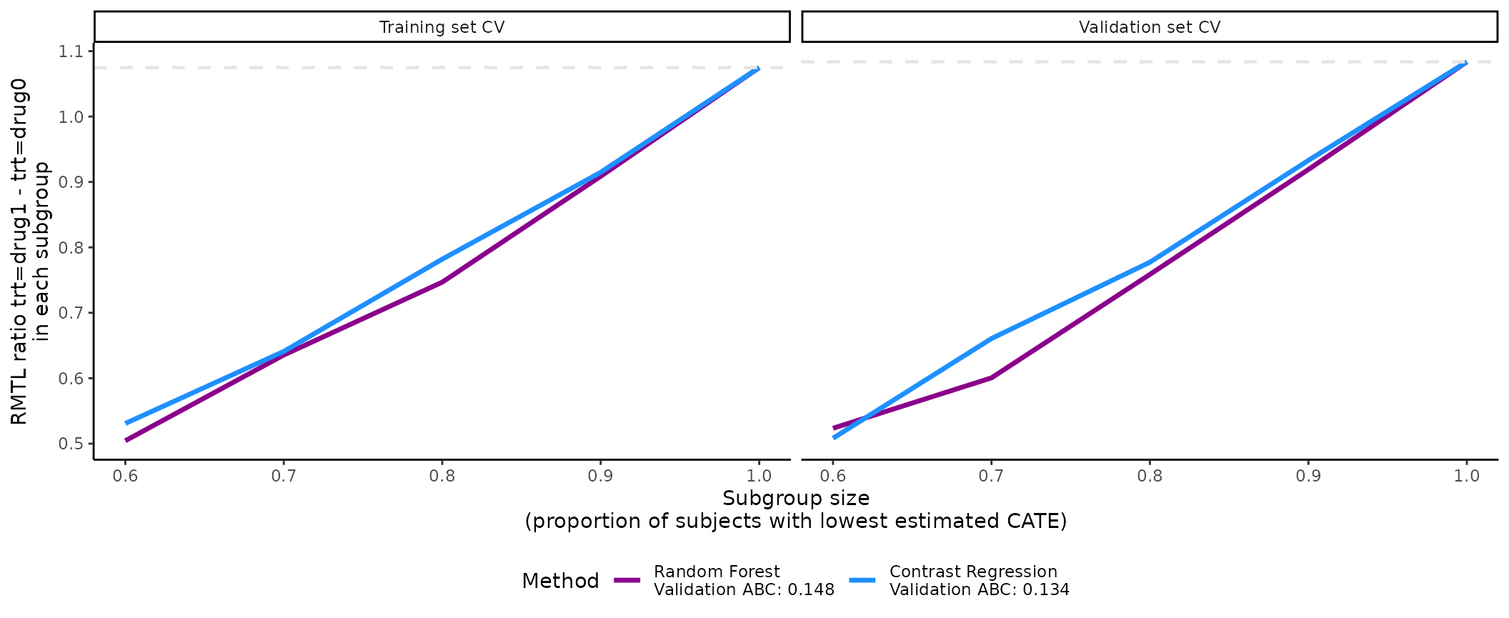

For this toy example, the methods are performing well in the training data as per the steep, increasing slopes on the left plot. Moreover, all methods generalize well to the validation data, as indicated by the monotonous increasing curves in the validation data (right plot). The dashed gray line is the ATE in the entire data set, which is why all lines merge to this reference line when subgroup size is 100% of the data (prop.cutoff = 1). For more explanation on the validation curves, see the function description.

The plot’s legend includes the ABC statistics in the validation set. The user can choose to mute the ABC annotations by specifying show.abc = FALSE.

plot(x = output_catecv, 
     show.abc = FALSE, 
     ylab = c("RMTL ratio of drug1 vs drug0 in each subgroup"))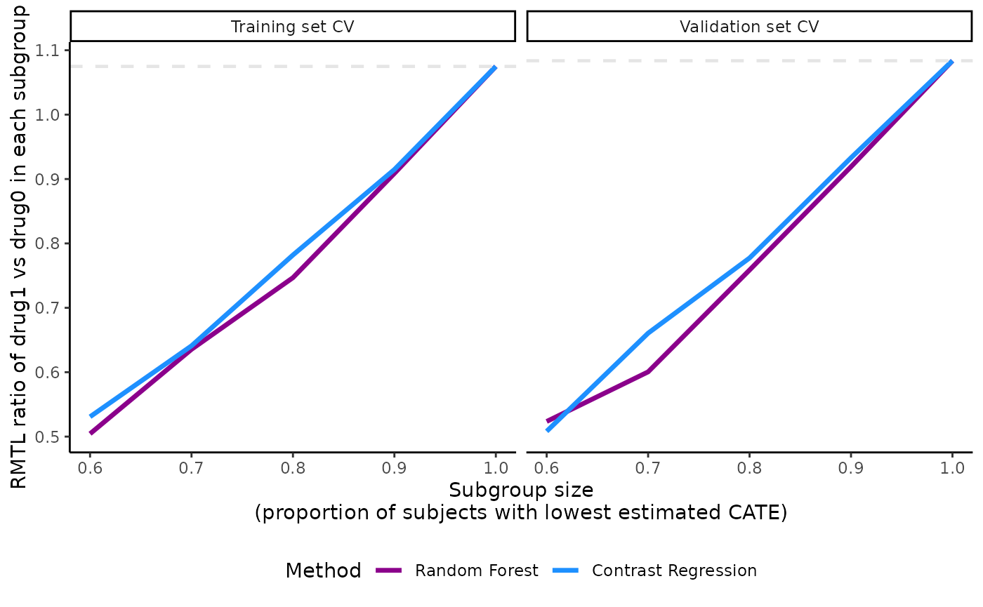

The user can choose to plot the validation curves of only 1 CV iteration instead of the average of all CV iterations. In the following example, we plot the validation curves of the second CV iteration by specifying cv.i = 2 and in grayscale by specifying grayscale = TRUE.

plot(x = output_catecv, 
     cv.i = 2, 
     grayscale = TRUE, 
     ylab = c("RMTL ratio of drug1 vs drug0 in each subgroup"))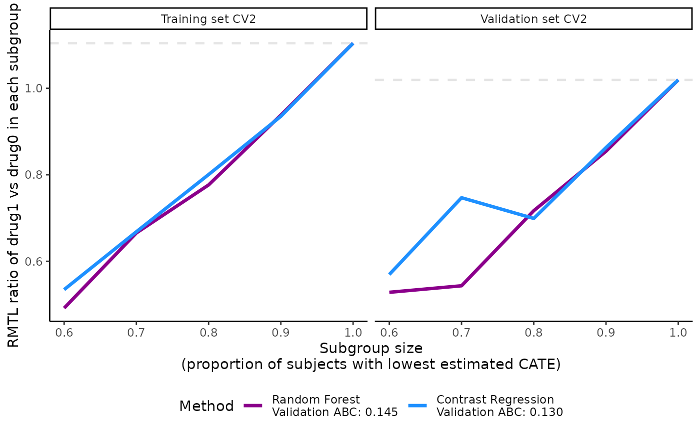

The user can also choose to use the median (instead of mean [default]) of the ATEs across CV iterations by specifying the argument combine = “median” in plot().

Visualization of the ATE in subgroups with `boxplot()`

The ATEs of multi-category subgroups that are mutually exclusive can be visualized as box plots, with 1 box plot for each scoring method. Only validation results are visualized here. The x-axis is determined by prop.multi and the y-axis is the estimated ATEs in each subgroup. We specify the ylab argument accordingly. The subgroups correspond to each row of the ate.est.valid.group.cv result in output_catecv, so in this example the subgroups are patient with the 50% lowest (0-50%), middle 10% (50-60%), and highest 40% (60-100%) estimated CATE scores. Notice that the groups do not have to be equally spaced in terms of percentiles. The box plot shows the distribution of the ATEs over all cv.n CV iterations, instead of a summary statistics like mean or median in plot().

boxplot(x = output_catecv,
        ylab = "RMTL ratio of drug1 vs drug0 in each subgroup")
#> Warning: Removed 4 rows containing non-finite outside the scale range
#> (`stat_boxplot()`).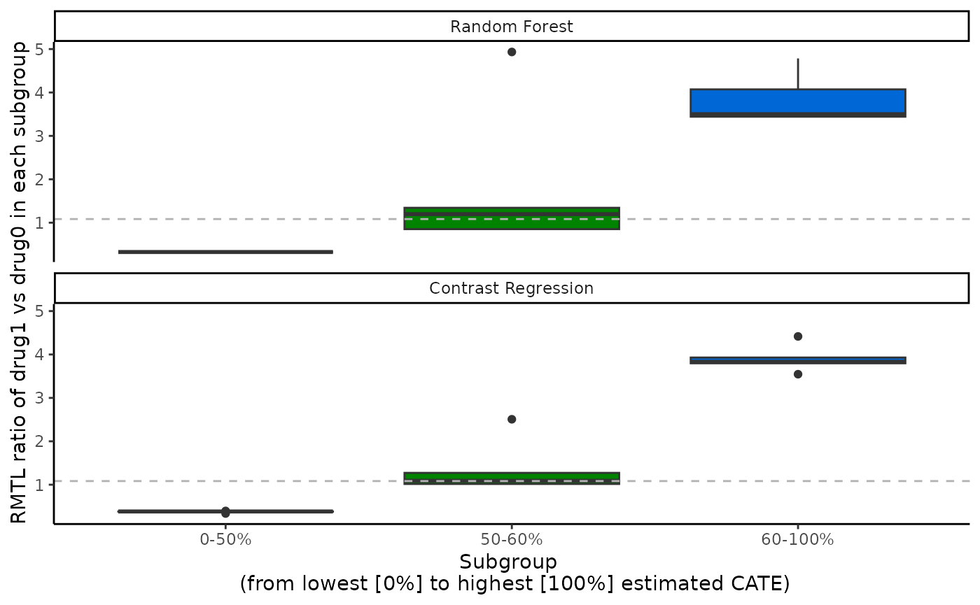

For this toy example, we can see why random forest and contrast regression methods have the 2 highest ABC and perform the best in the validation curves in the previous sections. They both have the most distinctive decreasing RMT ratio as we go from the subgroup with the 50% lowest CATE scores (red) to subgroup with the 40% highest CATE scores (blue). This implies that there is some evidence of heterogeneous treatment effect and that the CATE scores estimated with random forest or contrast regression can capture it. They also have relatively smaller variation as the boxes are thinner. In comparison, the other 3 methods also present this increasing trend in the box plots, but we observe a larger variation in the RMTL ratio, especially with boosting. We can see that the box plots correspond to the other 2 outputs, abc() and plot(). Note that the y-axis can have different scales for different scoring methods.

So far we provided 3 different metrics to summarize, visualize, and evaluate the catecv() outputs. The user is encouraged to choose their own way of data wrangling that fits to their particular situation.

Other `precmed` vignettes in this serie

1. Examples for count outcome
2. Examples for survival outcome
3. Additional examples
4. Theoretical details

Examples for survival outcome

Vignette 2 of 4

October 06, 2024

precmed: Precision Medicine in R

Examples with survival outcome of the entire workflow

Load required packages

Load data set (Example data with survival outcome)

Estimation of the ATE with `atefit()`

Estimation of the CATE score with `catefit()`

Internal validation via `catecv()`

Comparison of methods with `abc()`

Visualization of the validation curves with `plot()`

Visualization of the ATE in subgroups with `boxplot()`

Other `precmed` vignettes in this serie

Examples for survival outcome

Vignette 2 of 4

October 06, 2024

precmed: Precision Medicine in R

Examples with survival outcome of the entire workflow

Load required packages

Load data set (Example data with survival outcome)

Estimation of the ATE with atefit()

Estimation of the CATE score with catefit()

Internal validation via catecv()

Comparison of methods with abc()

Visualization of the validation curves with plot()

Visualization of the ATE in subgroups with boxplot()

Other precmed vignettes in this serie

Estimation of the ATE with `atefit()`

Estimation of the CATE score with `catefit()`

Internal validation via `catecv()`

Comparison of methods with `abc()`

Visualization of the validation curves with `plot()`

Visualization of the ATE in subgroups with `boxplot()`

Other `precmed` vignettes in this serie