library(bipd)
ds <- generate_ipdma_example(type = "continuous")9 Prediction of individual treatment effect using data from multiple studies
Orestis Efthimiou 
In this chapter, we discuss statistical methods for developing models to predict patient-level treatment effects using data from multiple randomized and non-randomized studies. We will first present prediction models that assume a constant treatment effect and discuss how to address heterogeneity in baseline risk. Subsequently, we will discuss approaches that allow for treatment effect modification by adopting two different approaches in an IPD-MA context, namely the risk modelling and the effect modelling approach. For both approaches, we will first discuss how to combine IPD from RCTs comparing the same two treatments. We will then discuss how these methods can be extended to include randomized data from multiple treatments, real-world data, and published aggregate data. We will discuss statistical software to implement these approaches and provide example code as supporting information. Real examples will be used throughout to illustrate the main methods.
9.1 Estimating heterogeneous treatment effects in pairwise meta-analysis
We hereby provide code for estimating patient-level treatment effects for the case when we have patient-level data from multiple randomized trials.
9.1.1 Example of a continuous outcome
9.1.1.1 Setup
We start by simulating an artificial dataset using the R package bipd:
Let us have a look at the dataset:
head(ds) studyid treat z1 z2 y
1 1 1 0.2352504 -1.37827118 6
2 1 0 0.1353785 0.04223993 11
3 1 1 0.7102602 -0.13908840 7
4 1 0 0.4373988 0.32715801 11
5 1 1 -1.3243928 -0.16398433 8
6 1 0 -1.1263310 0.65883970 11The simulated dataset contains information on the following variables:
- the trial indicator
studyid - the treatment indicator
treat, which takes the values 0 for control and 1 for active treatment - two prognostic variables
z1andz2 - the continuous outcome
y
| 0 (N=310) |
1 (N=290) |
Overall (N=600) |
|
|---|---|---|---|
| z1 | |||
| Mean (SD) | 0.0669 (0.999) | -0.0530 (1.06) | 0.00896 (1.03) |
| Median [Min, Max] | 0.123 [-3.02, 3.27] | -0.0786 [-3.52, 2.93] | 0.0405 [-3.52, 3.27] |
| z2 | |||
| Mean (SD) | 0.139 (0.970) | -0.0529 (1.03) | 0.0460 (1.00) |
| Median [Min, Max] | 0.167 [-2.50, 2.52] | -0.0493 [-2.66, 2.37] | 0.0603 [-2.66, 2.52] |
| studyid | |||
| 1 | 53 (17.1%) | 47 (16.2%) | 100 (16.7%) |
| 2 | 45 (14.5%) | 55 (19.0%) | 100 (16.7%) |
| 3 | 57 (18.4%) | 43 (14.8%) | 100 (16.7%) |
| 4 | 52 (16.8%) | 48 (16.6%) | 100 (16.7%) |
| 5 | 54 (17.4%) | 46 (15.9%) | 100 (16.7%) |
| 6 | 49 (15.8%) | 51 (17.6%) | 100 (16.7%) |
9.1.1.2 Model fitting
We synthesize the evidence using a Bayesian random effects meta-analysis model. The model is given in Equation 16.7 of the book. First we need set up the data and create the model:
ipd <- with(ds, ipdma.model.onestage(y = y, study = studyid, treat = treat,
                                     X = cbind(z1, z2),
                                     response = "normal",
                                     shrinkage = "none"),
                                     type = "random")
The JAGS model can be accessed as follows:
ipd$model.JAGSfunction ()
{
for (i in 1:Np) {
y[i] ~ dnorm(mu[i], sigma)
mu[i] <- alpha[studyid[i]] + inprod(beta[], X[i, ]) +
(1 - equals(treat[i], 1)) * inprod(gamma[], X[i,
]) + d[studyid[i], treat[i]]
}
sigma ~ dgamma(0.001, 0.001)
for (j in 1:Nstudies) {
d[j, 1] <- 0
d[j, 2] ~ dnorm(delta[2], tau)
}
sd ~ dnorm(0, 1)
T(0, )
tau <- pow(sd, -2)
delta[1] <- 0
delta[2] ~ dnorm(0, 0.001)
for (j in 1:Nstudies) {
alpha[j] ~ dnorm(0, 0.001)
}
for (k in 1:Ncovariate) {
beta[k] ~ dnorm(0, 0.001)
}
for (k in 1:Ncovariate) {
gamma[k] ~ dnorm(0, 0.001)
}
}
<environment: 0x59cdd7f580a8>We can fit the treatment effect model as follows:
samples <- ipd.run(ipd, n.chains = 2, n.iter = 20,
                   pars.save = c("alpha", "beta", "delta", "sd", "gamma"))
trtbenefit <- round(treatment.effect(ipd, samples, newpatient = c(z1 = 1, z2 = 0.5)), 2)
Here are the estimated model parameters:
summary(samples)
Iterations = 2001:2020
Thinning interval = 1
Number of chains = 2
Sample size per chain = 20

1. Empirical mean and standard deviation for each variable,
   plus standard error of the mean:

            Mean      SD Naive SE Time-series SE
alpha[1] 10.8767 0.05291 0.008366       0.015046
alpha[2]  7.9788 0.04971 0.007860       0.013831
alpha[3] 10.4453 0.04834 0.007644       0.011319
alpha[4]  9.6510 0.05113 0.008084       0.010348
alpha[5] 12.8748 0.05280 0.008348       0.011562
alpha[6] 15.8264 0.04291 0.006785       0.005829
beta[1]   0.1876 0.02156 0.003409       0.004529
beta[2]   0.2988 0.02084 0.003295       0.004911
delta[1]  0.0000 0.00000 0.000000       0.000000
delta[2] -2.7881 0.41407 0.065470       0.066031
gamma[1] -0.4913 0.02785 0.004403       0.004415
gamma[2]  0.5609 0.02707 0.004281       0.007673
sd        1.5939 0.33979 0.053726       0.045833

2. Quantiles for each variable:

            2.5%     25%     50%     75%   97.5%
alpha[1] 10.7929 10.8501 10.8722 10.9053 10.9774
alpha[2]  7.8836  7.9512  7.9798  8.0055  8.0836
alpha[3] 10.3619 10.4148 10.4494 10.4753 10.5278
alpha[4]  9.5816  9.6147  9.6446  9.6756  9.7476
alpha[5] 12.7855 12.8366 12.8789 12.9145 12.9509
alpha[6] 15.7454 15.7959 15.8318 15.8544 15.9012
beta[1]   0.1547  0.1739  0.1884  0.2011  0.2295
beta[2]   0.2624  0.2819  0.3018  0.3136  0.3319
delta[1]  0.0000  0.0000  0.0000  0.0000  0.0000
delta[2] -3.5437 -2.9984 -2.7723 -2.5662 -1.9535
gamma[1] -0.5448 -0.5055 -0.4886 -0.4747 -0.4466
gamma[2]  0.5169  0.5430  0.5552  0.5798  0.6186
sd        0.9888  1.3583  1.5950  1.7864  2.2002
9.1.1.3 Prection
We can now predict the individualized treatment effect for a new patient with covariate values z1 = 1 and z2 = 0.5.
round(treatment.effect(ipd, samples, newpatient = c(z1 = 1, z2 = 0.5)), 2)0.025 0.5 0.975
-3.76 -3.01 -2.16 This means that the predicted outcome for patient with covariate values z1 = 1 and z2 = 0.5 will differ by -3.01 units when receiving the active treatment (treat = 1) as compared to the control treatment (treat = 0).
We can also predict treatment benefit for all patients in the sample, and look at the distribution of predicted benefit.
library(dplyr)
library(ggplot2)

ds <- ds %>% mutate(benefit = NA,
                    study = paste("Trial", studyid))

for (i in seq(nrow(ds))) {
  newpat <- as.matrix(ds[i, c("z1", "z2")])
  ds$benefit[i] <- treatment.effect(ipd, samples, newpatient = newpat)["0.5"]
}

summbenefit <- ds %>% group_by(study) %>%
  summarize(mediabenefit = median(benefit), meanbenefit = mean(benefit))

ggplot(ds, aes(x = benefit)) +
  geom_histogram(aes(y = after_stat(density)), alpha = 0.3) +
  geom_density() +
  geom_vline(data = summbenefit, aes(xintercept = meanbenefit),
             linewidth = 0.5, lty = 2) +
  facet_wrap(~study) +
  ylab("Density") +
  xlab("Predicted treatment benefit")  + theme_bw()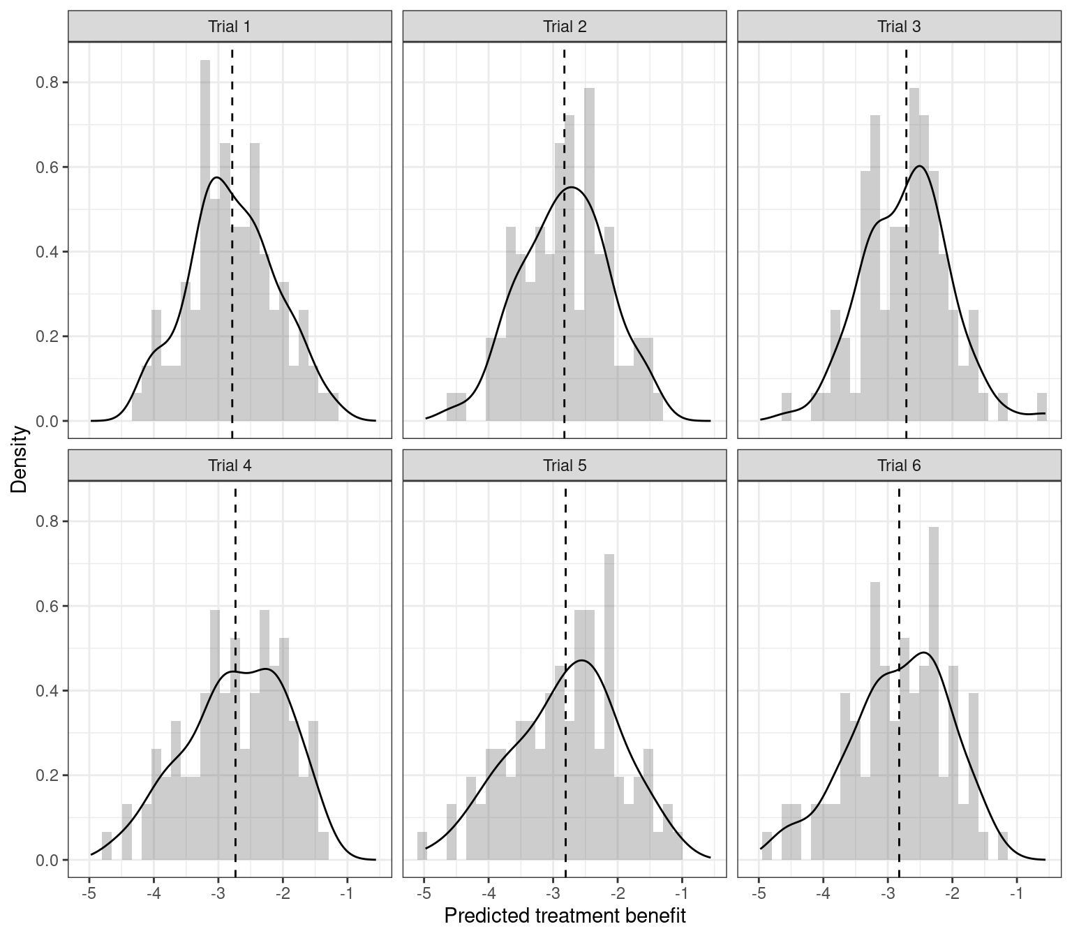
9.1.1.4 Penalization
Let us repeat the analysis, but this time while penalizing the treatment-covariate coefficients using a Bayesian LASSO prior.
ipd <- with(ds, ipdma.model.onestage(y = y, study = studyid,
                                     treat = treat,
                                     X = cbind(z1, z2),
                                     response = "normal",
                                     shrinkage = "laplace"),
            type = "random")

samples <- ipd.run(ipd, n.chains = 2, n.iter = 20,
                   pars.save = c("alpha", "beta", "delta", "sd", "gamma"))
Compiling model graph
Resolving undeclared variables
Allocating nodes
Graph information:
Observed stochastic nodes: 600
Unobserved stochastic nodes: 20
Total graph size: 6039
Initializing modelround(treatment.effect(ipd, samples, newpatient = c(1,0.5)), 2)0.025 0.5 0.975
-4.16 -2.85 -1.70 9.1.2 Example of a binary outcome
9.1.2.1 Setup
We now present the case of a binary outcome. We first generate a dataset as before, using the bipd package.
ds2 <- generate_ipdma_example(type = "binary")
head(ds2)
studyid treat w1 w2 y
1 1 0 0.6925323 -1.32369975 1
2 1 1 -0.7199908 0.43599379 1
3 1 1 0.2979550 -0.54827475 0
4 1 0 0.7126139 1.31520153 0
5 1 1 -1.1323112 -2.77408642 0
6 1 0 -1.6005528 -0.03296225 1The simulated dataset contains information on the following variables:
- the trial indicator
studyid - the treatment indicator
treat, which takes the values 0 for control and 1 for active treatment - two prognostic variables
w1andw2 - the binary outcome
y
| 0 (N=304) |
1 (N=296) |
Overall (N=600) |
|
|---|---|---|---|
| w1 | |||
| Mean (SD) | -0.0378 (1.05) | -0.0368 (1.01) | -0.0373 (1.03) |
| Median [Min, Max] | -0.0703 [-2.98, 2.39] | -0.125 [-2.44, 3.06] | -0.103 [-2.98, 3.06] |
| w2 | |||
| Mean (SD) | -0.00620 (1.03) | -0.0424 (1.11) | -0.0241 (1.07) |
| Median [Min, Max] | -0.00439 [-2.49, 3.02] | -0.0127 [-2.99, 3.18] | -0.0127 [-2.99, 3.18] |
| studyid | |||
| 1 | 53 (17.4%) | 47 (15.9%) | 100 (16.7%) |
| 2 | 56 (18.4%) | 44 (14.9%) | 100 (16.7%) |
| 3 | 49 (16.1%) | 51 (17.2%) | 100 (16.7%) |
| 4 | 48 (15.8%) | 52 (17.6%) | 100 (16.7%) |
| 5 | 51 (16.8%) | 49 (16.6%) | 100 (16.7%) |
| 6 | 47 (15.5%) | 53 (17.9%) | 100 (16.7%) |
9.1.2.2 Model fitting
We use a Bayesian random effects model with binomial likelihood. This is similar to the model 16.7 of the book, but with a Binomial likelihood, i.e.
\[ y_{ij}\sim \text{Binomial}(\pi_{ij}) \\ \] \[ \text{logit}(\pi_{ij})=a_j+\delta_j t_{ij}+ \sum_{l=1}^{L}\beta_l x_{ij}+ \sum_{l=1}^{L}\gamma_l x_{ij} t_{ij} \] The remaining of the model is as in the book. We can penalize the estimated parameters for effect modification (\(\gamma\)’s), using a Bayesian LASSO. We can do this using again the bipd package:
ipd2 <- with(ds2, ipdma.model.onestage(y = y, study = studyid, treat = treat,
                                       X = cbind(w1, w2),
                                       response = "binomial",
                                       shrinkage = "laplace"),
             type = "random", hy.prior = list("dunif", 0, 1))

ipd2$model.JAGS
function ()
{
for (i in 1:Np) {
y[i] ~ dbern(p[i])
logit(p[i]) <- alpha[studyid[i]] + inprod(beta[], X[i,
]) + (1 - equals(treat[i], 1)) * inprod(gamma[],
X[i, ]) + d[studyid[i], treat[i]]
}
for (j in 1:Nstudies) {
d[j, 1] <- 0
d[j, 2] ~ dnorm(delta[2], tau)
}
sd ~ dnorm(0, 1)
T(0, )
tau <- pow(sd, -2)
delta[1] <- 0
delta[2] ~ dnorm(0, 0.001)
for (j in 1:Nstudies) {
alpha[j] ~ dnorm(0, 0.001)
}
for (k in 1:Ncovariate) {
beta[k] ~ dnorm(0, 0.001)
}
tt <- lambda
lambda <- pow(lambda.inv, -1)
lambda.inv ~ dunif(0, 5)
for (k in 1:Ncovariate) {
gamma[k] ~ ddexp(0, tt)
}
}
<environment: 0x59cddb63b758>samples <- ipd.run(ipd2, n.chains = 2, n.iter = 20,
pars.save = c("alpha", "beta", "delta", "sd", "gamma"))
summary(samples)
Iterations = 2001:2020
Thinning interval = 1
Number of chains = 2
Sample size per chain = 20

1. Empirical mean and standard deviation for each variable,
   plus standard error of the mean:

             Mean     SD Naive SE Time-series SE
alpha[1] -0.26139 0.1779  0.02813        0.02725
alpha[2] -1.02758 0.2607  0.04122        0.06840
alpha[3] -0.67582 0.2674  0.04228        0.06891
alpha[4] -0.59390 0.3215  0.05083        0.07254
alpha[5] -0.52414 0.3189  0.05042        0.08469
alpha[6] -0.83367 0.2691  0.04256        0.06675
beta[1]   0.15337 0.1051  0.01662        0.01442
beta[2]   0.07604 0.1305  0.02064        0.02977
delta[1]  0.00000 0.0000  0.00000        0.00000
delta[2] -0.19495 0.3718  0.05879        0.07694
gamma[1]  0.02270 0.1416  0.02239        0.02931
gamma[2]  0.03300 0.1315  0.02080        0.03792
sd        0.71952 0.2068  0.03269        0.05364

2. Quantiles for each variable:

              2.5%      25%      50%      75%    97.5%
alpha[1] -0.635416 -0.37037 -0.26158 -0.16425  0.05838
alpha[2] -1.494488 -1.23506 -1.01694 -0.81253 -0.61791
alpha[3] -1.097759 -0.87491 -0.72970 -0.46869 -0.24013
alpha[4] -1.082326 -0.81977 -0.62738 -0.44397  0.09548
alpha[5] -1.170170 -0.68283 -0.51475 -0.33748  0.05015
alpha[6] -1.266977 -1.00267 -0.86315 -0.65258 -0.40608
beta[1]  -0.004993  0.08293  0.13440  0.21470  0.33910
beta[2]  -0.110911 -0.04075  0.07981  0.17575  0.30610
delta[1]  0.000000  0.00000  0.00000  0.00000  0.00000
delta[2] -0.943654 -0.42304 -0.14353  0.03852  0.38097
gamma[1] -0.228256 -0.04570  0.02463  0.07360  0.33308
gamma[2] -0.258714 -0.02196  0.06827  0.12229  0.24545
sd        0.364509  0.57552  0.69493  0.87975  1.08048
The predicted treatment benefit for a new patient with covariates w1 = 1.6 and w2 = 1.3 is given as:
round(treatment.effect(ipd2, samples, newpatient = c(w1 = 1.6, w2 = 1.3)), 2)0.025 0.5 0.975
0.34 0.87 1.91 In other words, the aforementioned patient 0.87 (95% Credibility Interval: 0.34 to 1.91)
9.2 Estimating heterogeous treatment effects in network meta-analysis
9.2.1 Example of a continuous outcome
9.2.1.1 Setup
We use again the bipd package to simulate a dataset:
ds3 <- generate_ipdnma_example(type = "continuous")
head(ds3)
studyid treat z1 z2 y
1 1 2 -0.09713174 1.4766550 10
2 1 2 -0.57214805 -1.4315506 7
3 1 2 -0.05707383 -0.9623695 7
4 1 1 -1.07935434 0.2140941 11
5 1 1 1.72837498 0.2984847 11
6 1 1 0.09060760 0.9888786 11Let us look into the data a bit in more detail:
| 1 (N=353) |
2 (N=349) |
3 (N=298) |
Overall (N=1000) |
|
|---|---|---|---|---|
| z1 | ||||
| Mean (SD) | 0.0795 (0.953) | -0.0477 (0.954) | -0.0256 (0.962) | 0.00377 (0.957) |
| Median [Min, Max] | 0.0723 [-3.01, 3.29] | -0.0285 [-2.46, 2.50] | -0.000102 [-2.80, 2.33] | 0.0197 [-3.01, 3.29] |
| z2 | ||||
| Mean (SD) | 0.0343 (0.998) | -0.0683 (0.957) | 0.00557 (0.930) | -0.0101 (0.964) |
| Median [Min, Max] | 0.0173 [-3.14, 2.69] | -0.118 [-2.75, 2.16] | 0.0463 [-2.64, 2.64] | -0.0127 [-3.14, 2.69] |
| studyid | ||||
| 1 | 52 (14.7%) | 48 (13.8%) | 0 (0%) | 100 (10.0%) |
| 2 | 49 (13.9%) | 51 (14.6%) | 0 (0%) | 100 (10.0%) |
| 3 | 50 (14.2%) | 50 (14.3%) | 0 (0%) | 100 (10.0%) |
| 4 | 49 (13.9%) | 0 (0%) | 51 (17.1%) | 100 (10.0%) |
| 5 | 48 (13.6%) | 0 (0%) | 52 (17.4%) | 100 (10.0%) |
| 6 | 0 (0%) | 51 (14.6%) | 49 (16.4%) | 100 (10.0%) |
| 7 | 0 (0%) | 52 (14.9%) | 48 (16.1%) | 100 (10.0%) |
| 8 | 24 (6.8%) | 36 (10.3%) | 40 (13.4%) | 100 (10.0%) |
| 9 | 47 (13.3%) | 29 (8.3%) | 24 (8.1%) | 100 (10.0%) |
| 10 | 34 (9.6%) | 32 (9.2%) | 34 (11.4%) | 100 (10.0%) |
9.2.1.2 Model fitting
We will use the model shown in Equation 16.8 in the book. In addition, we will use Bayesian LASSO to penalize the treatment-covariate interactions.
ipd3 <- with(ds3, ipdnma.model.onestage(y = y, study = studyid, treat = treat,
                                        X = cbind(z1, z2),
                                        response = "normal",
                                        shrinkage = "laplace",
                                        type = "random"))
ipd3$model.JAGS
function ()
{
for (i in 1:Np) {
y[i] ~ dnorm(mu[i], sigma)
mu[i] <- alpha[studyid[i]] + inprod(beta[], X[i, ]) +
inprod(gamma[treat[i], ], X[i, ]) + d[studyid[i],
treatment.arm[i]]
}
sigma ~ dgamma(0.001, 0.001)
for (i in 1:Nstudies) {
w[i, 1] <- 0
d[i, 1] <- 0
for (k in 2:na[i]) {
d[i, k] ~ dnorm(mdelta[i, k], taudelta[i, k])
mdelta[i, k] <- delta[t[i, k]] - delta[t[i, 1]] +
sw[i, k]
taudelta[i, k] <- tau * 2 * (k - 1)/k
w[i, k] <- d[i, k] - delta[t[i, k]] + delta[t[i,
1]]
sw[i, k] <- sum(w[i, 1:(k - 1)])/(k - 1)
}
}
sd ~ dnorm(0, 1)
T(0, )
tau <- pow(sd, -2)
delta[1] <- 0
for (k in 2:Ntreat) {
delta[k] ~ dnorm(0, 0.001)
}
for (j in 1:Nstudies) {
alpha[j] ~ dnorm(0, 0.001)
}
for (k in 1:Ncovariate) {
beta[k] ~ dnorm(0, 0.001)
}
lambda[1] <- 0
lambda.inv[1] <- 0
for (m in 2:Ntreat) {
tt[m] <- lambda[m] * sigma
lambda[m] <- pow(lambda.inv[m], -1)
lambda.inv[m] ~ dunif(0, 5)
}
for (k in 1:Ncovariate) {
gamma[1, k] <- 0
for (m in 2:Ntreat) {
gamma[m, k] ~ ddexp(0, tt[m])
}
}
}
<environment: 0x59cddb365d70>samples <- ipd.run(ipd3, n.chains = 2, n.iter = 20,
pars.save = c("alpha", "beta", "delta", "sd", "gamma"))Compiling model graph
Resolving undeclared variables
Allocating nodes
Graph information:
Observed stochastic nodes: 1000
Unobserved stochastic nodes: 35
Total graph size: 10141
Initializing modelsummary(samples)
Iterations = 2001:2020
Thinning interval = 1
Number of chains = 2
Sample size per chain = 20

1. Empirical mean and standard deviation for each variable,
   plus standard error of the mean:

              Mean      SD Naive SE Time-series SE
alpha[1]   10.9940 0.04867 0.007696       0.011341
alpha[2]    8.0234 0.05581 0.008825       0.017836
alpha[3]   10.5663 0.04543 0.007183       0.009628
alpha[4]    9.6417 0.04719 0.007461       0.008469
alpha[5]   12.8774 0.03981 0.006295       0.006638
alpha[6]   13.2658 0.04265 0.006743       0.006323
alpha[7]    7.4408 0.03978 0.006290       0.006453
alpha[8]   11.2500 0.05534 0.008749       0.015319
alpha[9]   10.1340 0.03568 0.005641       0.007555
alpha[10]   9.1532 0.04592 0.007260       0.006907
beta[1]     0.1918 0.01581 0.002499       0.003902
beta[2]     0.2817 0.01565 0.002475       0.002745
delta[1]    0.0000 0.00000 0.000000       0.000000
delta[2]   -3.0145 0.04880 0.007716       0.013146
delta[3]   -1.1946 0.06758 0.010686       0.010824
gamma[1,1]  0.0000 0.00000 0.000000       0.000000
gamma[2,1] -0.5585 0.02349 0.003715       0.007680
gamma[3,1] -0.3305 0.02624 0.004149       0.006997
gamma[1,2]  0.0000 0.00000 0.000000       0.000000
gamma[2,2]  0.5777 0.03182 0.005031       0.007687
gamma[3,2]  0.3859 0.01987 0.003142       0.003868
sd          0.1519 0.03583 0.005666       0.006339

2. Quantiles for each variable:

               2.5%     25%     50%     75%   97.5%
alpha[1]   10.89408 10.9623 10.9995 11.0359 11.0644
alpha[2]    7.92410  7.9900  8.0286  8.0541  8.1230
alpha[3]   10.48169 10.5402 10.5612 10.5954 10.6492
alpha[4]    9.53989  9.6146  9.6438  9.6779  9.7119
alpha[5]   12.82137 12.8495 12.8667 12.9073 12.9569
alpha[6]   13.17735 13.2425 13.2625 13.2928 13.3394
alpha[7]    7.37394  7.4166  7.4342  7.4632  7.5392
alpha[8]   11.15071 11.2084 11.2509 11.2779 11.3599
alpha[9]   10.06136 10.1125 10.1345 10.1571 10.2061
alpha[10]   9.04498  9.1216  9.1595  9.1871  9.2268
beta[1]     0.16184  0.1810  0.1916  0.2023  0.2185
beta[2]     0.24221  0.2743  0.2829  0.2926  0.3089
delta[1]    0.00000  0.0000  0.0000  0.0000  0.0000
delta[2]   -3.09850 -3.0486 -3.0132 -2.9824 -2.9127
delta[3]   -1.30246 -1.2339 -1.1966 -1.1756 -1.0564
gamma[1,1]  0.00000  0.0000  0.0000  0.0000  0.0000
gamma[2,1] -0.61075 -0.5729 -0.5587 -0.5412 -0.5230
gamma[3,1] -0.37654 -0.3502 -0.3314 -0.3081 -0.2880
gamma[1,2]  0.00000  0.0000  0.0000  0.0000  0.0000
gamma[2,2]  0.53049  0.5606  0.5774  0.5847  0.6587
gamma[3,2]  0.35963  0.3718  0.3817  0.3960  0.4281
sd          0.09181  0.1281  0.1503  0.1825  0.2069
As before, we can use the treatment.effect() function of bipd to estimate relative effects for new patients.
treatment.effect(ipd3, samples, newpatient= c(1,2))$`treatment 2`
0.025 0.5 0.975
-2.539919 -2.395889 -2.220652
$`treatment 3`
0.025 0.5 0.975
-0.8553820 -0.7376539 -0.5482169 This gives us the relative effects for all treatments versus the reference. To obtain relative effects between active treatments we need some more coding:
samples.all=data.frame(rbind(samples[[1]], samples[[2]]))
newpatient= c(1,2)
newpatient <- (newpatient - ipd3$scale_mean)/ipd3$scale_sd

median(
  samples.all$delta.2.+samples.all$gamma.2.1.*
    newpatient[1]+samples.all$gamma.2.2.*newpatient[2]
-
  (samples.all$delta.3.+samples.all$gamma.3.1.*newpatient[1]+
     samples.all$gamma.3.2.*newpatient[2])
)
[1] -1.653063quantile(samples.all$delta.2.+samples.all$gamma.2.1.*
newpatient[1]+samples.all$gamma.2.2.*newpatient[2]
-(samples.all$delta.3.+samples.all$gamma.3.1.*newpatient[1]+
samples.all$gamma.3.2.*newpatient[2])
, probs = 0.025) 2.5%
-1.80513 quantile(samples.all$delta.2.+samples.all$gamma.2.1.*
newpatient[1]+samples.all$gamma.2.2.*newpatient[2]
-(samples.all$delta.3.+samples.all$gamma.3.1.*newpatient[1]+
samples.all$gamma.3.2.*newpatient[2])
, probs = 0.975) 97.5%
-1.533038 9.2.2 Modeling patient-level relative effects using randomized and observational evidence for a network of treatments
We will now follow Chapter 16.3.5 from the book. In this analysis we will not use penalization, and we will assume fixed effects. For an example with penalization and random effects, see part 2 of this vignettte.
9.2.2.1 Setup
We generate a very simple dataset of three studies comparing three treatments. We will assume 2 RCTs and 1 non-randomized trial:
ds4 <- generate_ipdnma_example(type = "continuous")
ds4 <- ds4 %>% filter(studyid %in% c(1,4,10)) %>%
  mutate(studyid = factor(studyid) %>%
           recode_factor(
             "1" = "1",
             "4" = "2",
             "10" = "3"),
         design = ifelse(studyid == "3", "nrs", "rct"))
The sample size is as follows:
           s1 s2 s3
  treat A: 46 57 33
  treat B: 54  0 40
  treat C:  0 43 27
9.2.2.2 Model fitting
We will use the design-adjusted model, equation 16.9 in the book. We will fit a two-stage fixed effects meta-analysis and we will use a variance inflation factor. The code below is used to specify the analysis of each individual study. Briefly, in each study we adjust the treatment effect for the prognostic factors z1 and z2, as well as their interaction with treat.
library(rjags)Loading required package: codaLinked to JAGS 4.3.0Loaded modules: basemod,bugsfirst.stage <- "
model{
for (i in 1:N){
y[i] ~ dnorm(mu[i], tau)
mu[i] <- a + inprod(b[], X[i,]) + inprod(c[,treat[i]], X[i,]) + d[treat[i]]
}
sigma ~ dunif(0, 5)
tau <- pow(sigma, -2)
a ~ dnorm(0, 0.001)
for(k in 1:Ncovariate){
b[k] ~ dnorm(0,0.001)
}
for(k in 1:Ncovariate){
c[k,1] <- 0
}
tauGamma <- pow(sdGamma,-1)
sdGamma ~ dunif(0, 5)
for(k in 1:Ncovariate){
for(t in 2:Ntreat){
c[k,t] ~ ddexp(0, tauGamma)
}
}
d[1] <- 0
for(t in 2:Ntreat){
d[t] ~ dnorm(0, 0.001)
}
}"Subsequently, we estimate the relative treatment effects in the first (randomized) study comparing treatments A and B:
model1.spec <- textConnection(first.stage)
data1 <- with(ds4 %>% filter(studyid == 1),
              list(y = y,
                   N = length(y),
                   X = cbind(z1,z2),
                   treat = treat,
                   Ncovariate = 2,
                   Ntreat = 2))
jags.m <- jags.model(model1.spec, data = data1, n.chains = 2, n.adapt = 500,
                     quiet =  TRUE)
params <- c("d", "c")
samps4.1 <- coda.samples(jags.m, params, n.iter = 50)
samps.all.s1 <- data.frame(as.matrix(samps4.1))

samps.all.s1 <- samps.all.s1[, c("c.1.2.", "c.2.2.", "d.2.")]
delta.1 <- colMeans(samps.all.s1)
cov.1 <- var(samps.all.s1)
We repeat the analysis for the second (randomized) study comparing treatments A and C:
model1.spec <- textConnection(first.stage)
data2 <- with(ds4 %>% filter(studyid == 2),
              list(y = y,
                   N = length(y),
                   X = cbind(z1,z2),
                   treat = ifelse(treat == 3, 2, treat),
                   Ncovariate = 2,
                   Ntreat = 2))
jags.m <- jags.model(model1.spec, data = data2, n.chains = 2, n.adapt = 100,
                     quiet =  TRUE)
params <- c("d", "c")
samps4.2 <- coda.samples(jags.m, params, n.iter = 50)
samps.all.s2 <- data.frame(as.matrix(samps4.2))
samps.all.s2 <- samps.all.s2[, c("c.1.2.", "c.2.2.", "d.2.")]
delta.2 <- colMeans(samps.all.s2)
cov.2 <- var(samps.all.s2)
Finally, we analyze the third (non-randomized) study comparing treatments A, B, and C:
model1.spec <- textConnection(first.stage)
data3 <- with(ds4 %>% filter(studyid == 3),
              list(y = y,
                   N = length(y),
                   X = cbind(z1,z2),
                   treat = treat,
                   Ncovariate = 2,
                   Ntreat = 3))
jags.m <- jags.model(model1.spec, data = data3, n.chains = 2, n.adapt = 100,
                     quiet = TRUE)
params <- c("d", "c")
samps4.3 <- coda.samples(jags.m, params, n.iter = 50)
samps.all.s3 <- data.frame(as.matrix(samps4.3))

samps.all.s3 <- samps.all.s3[, c("c.1.2.", "c.2.2.", "d.2.", "c.1.3.",
                                 "c.2.3.", "d.3.")]
delta.3 <- colMeans(samps.all.s3)
cov.3 <- var(samps.all.s3)
The corresponding treatment effect estimates are depicted below:
| study | B versus A | C versus A |
|---|---|---|
| study 1 | -3.015 (SE = 0.056 ) | |
| study 2 | -1.082 (SE = 0.067 ) | |
| study 3 | -3.004 (SE = 0.068 ) | -0.966 (SE = 0.073 ) |
We can now fit the second stage of the network meta-analysis. The corresponding JAGS model is specified below:
second.stage <-
"model{

  #likelihood
  y1 ~ dmnorm(Mu1, Omega1)
  y2 ~ dmnorm(Mu2, Omega2)
  y3 ~ dmnorm(Mu3, Omega3*W)


  Omega1 <- inverse(cov.1)
  Omega2 <- inverse(cov.2)
  Omega3 <- inverse(cov.3)

  Mu1 <- c(gamma[,1], delta[2])
  Mu2 <- c(gamma[,2], delta[3])
  Mu3 <- c(gamma[,1], delta[2],gamma[,2], delta[3])

  #parameters
  for(i in 1:2){
    gamma[i,1] ~ dnorm(0, 0.001)
    gamma[i,2] ~ dnorm(0, 0.001)
  }

  delta[1] <- 0
  delta[2] ~ dnorm(0, 0.001)
  delta[3] ~ dnorm(0, 0.001)

}
"
We can fit as follows:
model1.spec <- textConnection(second.stage)
data3 <- list(y1 = delta.1, y2 = delta.2, y3 = delta.3,
              cov.1 = cov.1, cov.2 = cov.2, cov.3 = cov.3, W = 0.5)

jags.m <- jags.model(model1.spec, data = data3, n.chains = 2, n.adapt = 50,
                     quiet = TRUE)
params <- c("delta", "gamma")
samps4.3 <- coda.samples(jags.m, params, n.iter = 50)summary(samps4.3)
Iterations = 1:50
Thinning interval = 1
Number of chains = 2
Sample size per chain = 50

1. Empirical mean and standard deviation for each variable,
   plus standard error of the mean:

              Mean      SD Naive SE Time-series SE
delta[1]    0.0000 0.00000 0.000000       0.000000
delta[2]   -3.0618 0.06124 0.006124       0.006122
delta[3]   -1.0192 0.05227 0.005227       0.005640
gamma[1,1] -0.8052 0.03991 0.003991       0.003464
gamma[2,1]  0.8798 0.09015 0.009015       0.009048
gamma[1,2] -0.6018 0.04782 0.004782       0.005812
gamma[2,2]  0.4305 0.05521 0.005521       0.005549

2. Quantiles for each variable:

              2.5%     25%     50%     75%   97.5%
delta[1]    0.0000  0.0000  0.0000  0.0000  0.0000
delta[2]   -3.1782 -3.0970 -3.0640 -3.0261 -2.9678
delta[3]   -1.0944 -1.0615 -1.0211 -0.9781 -0.9290
gamma[1,1] -0.8854 -0.8321 -0.8052 -0.7788 -0.7204
gamma[2,1]  0.7876  0.8404  0.8703  0.9038  0.9775
gamma[1,2] -0.6849 -0.6325 -0.6118 -0.5723 -0.5042
gamma[2,2]  0.3161  0.4035  0.4339  0.4662  0.5211
# calculate treatment effects
samples.all = data.frame(rbind(samps4.3[[1]], samps4.3[[2]]))
newpatient = c(1,2)
median(
samples.all$delta.2. + samples.all$gamma.1.1.*newpatient[1] +
samples.all$gamma.2.1.*newpatient[2]
)[1] -2.121315quantile(samples.all$delta.2.+samples.all$gamma.1.1.*newpatient[1]+
samples.all$gamma.2.1.*newpatient[2]
, probs = 0.025) 2.5%
-2.389289 quantile(samples.all$delta.2.+samples.all$gamma.1.1.*newpatient[1]+
samples.all$gamma.2.1.*newpatient[2]
, probs = 0.975) 97.5%
-1.84765 Version info
This chapter was rendered using the following version of R and its packages:
R version 4.2.3 (2023-03-15)
Platform: x86_64-pc-linux-gnu (64-bit)
Running under: Ubuntu 22.04.4 LTS

Matrix products: default
BLAS:   /usr/lib/x86_64-linux-gnu/openblas-pthread/libblas.so.3
LAPACK: /usr/lib/x86_64-linux-gnu/openblas-pthread/libopenblasp-r0.3.20.so

locale:
 [1] LC_CTYPE=C.UTF-8       LC_NUMERIC=C           LC_TIME=C.UTF-8
 [4] LC_COLLATE=C.UTF-8     LC_MONETARY=C.UTF-8    LC_MESSAGES=C.UTF-8
 [7] LC_PAPER=C.UTF-8       LC_NAME=C              LC_ADDRESS=C
[10] LC_TELEPHONE=C         LC_MEASUREMENT=C.UTF-8 LC_IDENTIFICATION=C

attached base packages:
[1] stats     graphics  grDevices utils     datasets  methods   base

other attached packages:
[1] rjags_4-15       coda_0.19-4.1    ggplot2_3.5.0    bipd_0.3
[5] kableExtra_1.4.0 dplyr_1.1.4      table1_1.4.3

loaded via a namespace (and not attached):
 [1] highr_0.10        pillar_1.9.0      compiler_4.2.3    tools_4.2.3
 [5] digest_0.6.35     gtable_0.3.4      lattice_0.20-45   jsonlite_1.8.8
 [9] evaluate_0.23     lifecycle_1.0.4   tibble_3.2.1      viridisLite_0.4.2
[13] pkgconfig_2.0.3   rlang_1.1.3       cli_3.6.2         rstudioapi_0.15.0
[17] yaml_2.3.8        mvtnorm_1.2-4     xfun_0.42         fastmap_1.1.1
[21] withr_3.0.0       stringr_1.5.1     knitr_1.45        xml2_1.3.6
[25] generics_0.1.3    vctrs_0.6.5       htmlwidgets_1.6.4 systemfonts_1.0.6
[29] grid_4.2.3        tidyselect_1.2.1  svglite_2.1.3     glue_1.7.0
[33] R6_2.5.1          fansi_1.0.6       rmarkdown_2.26    Formula_1.2-5
[37] farver_2.1.1      magrittr_2.0.3    codetools_0.2-19  scales_1.3.0
[41] htmltools_0.5.7   colorspace_2.1-0  labeling_0.4.3    utf8_1.2.4
[45] stringi_1.8.3     munsell_0.5.0