Doubly robust estimator of and inference for the average treatment effect for survival data
Source:R/ATE_surv.R
atefitsurv.RdDoubly robust estimator of the average treatment effect between two treatments, which is the restricted mean time lost ratio for survival outcomes. Bootstrap is used for inference.
Usage
atefitsurv(
  data,
  cate.model,
  ps.model,
  ps.method = "glm",
  ipcw.model = NULL,
  ipcw.method = "breslow",
  minPS = 0.01,
  maxPS = 0.99,
  followup.time = NULL,
  tau0 = NULL,
  surv.min = 0.025,
  n.boot = 500,
  seed = NULL,
  verbose = 0
)
Arguments
- data
A data frame containing the variables in the outcome, propensity score, and inverse probability of censoring models (if specified); a data frame with
nrows (1 row per observation).- cate.model
A formula describing the outcome model to be fitted. The outcome must appear on the left-hand side. For survival outcomes, a
Survobject must be used to describe the outcome.- ps.model
A formula describing the propensity score (PS) model to be fitted. The treatment must appear on the left-hand side. The treatment must be a numeric vector coded as 0/1. If data are from a randomized controlled trial, specify
ps.model = ~1as an intercept-only model.- ps.method
A character value for the method to estimate the propensity score. Allowed values include one of:
'glm'for logistic regression with main effects only (default), or'lasso'for a logistic regression with main effects and LASSO penalization on two-way interactions (added to the model if interactions are not specified inps.model). Relevant only whenps.modelhas more than one variable.- ipcw.model
A formula describing the inverse probability of censoring weighting (IPCW) model to be fitted. The left-hand side must be empty. Only applies for survival outcomes. Default is
NULL, which corresponds to specifying the IPCW with the same covariates as the outcome modelcate.model, plus the treatment.- ipcw.method
A character value for the censoring model. Only applies for survival outcomes. Allowed values are:
'breslow'(Cox regression with Breslow estimator of t he baseline survivor function),'aft (exponential)','aft (weibull)','aft (lognormal)'or'aft (loglogistic)'(accelerated failure time model with different distributions for y variable). Default is'breslow'.- minPS
A numerical value (in `[0, 1]`) below which estimated propensity scores should be truncated. Default is
0.01.- maxPS
A numerical value (in `(0, 1]`) above which estimated propensity scores should be truncated. Must be strictly greater than
minPS. Default is0.99.- followup.time
A column name in
dataspecifying the maximum follow-up time, interpreted as the potential censoring time. Only applies for survival outcomes. Default isNULL, which corresponds to unknown potential censoring time.- tau0
The truncation time for defining restricted mean time lost. Only applies for survival outcomes. Default is
NULL, which corresponds to setting the truncation time as the maximum survival time in the data.- surv.min
Lower truncation limit for the probability of being censored. It must be a positive value and should be chosen close to 0. Only applies for survival outcomes. Default is
0.025.- n.boot
A numeric value indicating the number of bootstrap samples used. Default is
500.- seed
An optional integer specifying an initial randomization seed for reproducibility. Default is
NULL, corresponding to no seed.- verbose
An integer value indicating whether intermediate progress messages should be printed.
1indicates messages are printed and0otherwise. Default is0.
Value
Return an object of class atefit with 6 elements:
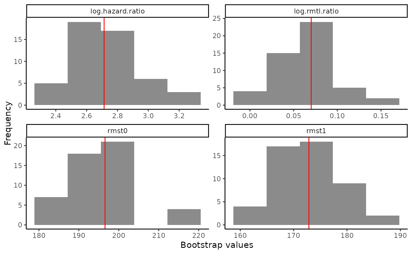
rmst1: A vector of numeric values of the estimated RMST, bootstrap standard error, lower and upper limits of 95% confidence interval, and the p-value in the grouptrt=1.rmst0: A vector of numeric values of the estimated RMST, bootstrap standard error, lower and upper limits of 95% confidence interval, and the p-value in the grouptrt=0.log.rmtl.ratio: A vector of numeric values of the estimated log RMTL ratio oftrt=1overtrt=0, bootstrap standard error, lower and upper limits of 95% confidence interval, and the p-value.log.hazard.ratio: A vector of numeric values of the estimated adjusted log hazard ratio oftrt=1overtrt=0, bootstrap standard error, lower and upper limits of 95% confidence interval, and the p-value.trt.boot: Estimates ofrmst1,rmst0,log.rmtl.ratioandlog.hazard.ratioin each bootstrap sample.warning: A warning message produced if the treatment variable was not coded as 0/1. The key to map the original coding of the variable to a 0/1 key is displayed in the warning to facilitate the interpretation of the remaining of the output.
Details
This helper function estimates the average treatment effect (ATE) for survival data between two treatment groups in a given dataset. The ATE is estimated with a doubly robust estimator that accounts for imbalances in covariate distributions between the two treatment groups with inverse probability treatment and censoring weighting. For survival outcomes, the estimated ATE is the estimated by RMTL ratio between treatment 1 versus treatment 0. The log-transformed ATEs and log-transformed adjusted hazard ratios are returned, as well as the estimated RMST in either treatment group. The variability of the estimated RMTL ratio is calculated using bootstrap. Additional outputs include standard error of the log RMTL ratio, 95% confidence interval, p-value, and a histogram of the bootstrap estimates.
Examples
# \donttest{
library(survival)
tau0 <- with(survivalExample,
             min(quantile(y[trt == "drug1"], 0.95), quantile(y[trt == "drug0"], 0.95)))

output <- atefitsurv(data = survivalExample,
                     cate.model = Surv(y, d) ~ age + female +
                                  previous_cost + previous_number_relapses,
                     ps.model = trt ~ age + previous_treatment,
                     tau0 = tau0,
                     n.boot = 50,
                     seed = 999,
                     verbose = 1)
#> Warning: Variable trt was recoded to 0/1 with drug0->0 and drug1->1.
#>
  |
  |                                                                      |   0%
  |
  |=                                                                     |   2%
  |
  |===                                                                   |   4%
  |
  |====                                                                  |   6%
  |
  |======                                                                |   8%
  |
  |=======                                                               |  10%
  |
  |=========                                                             |  12%
  |
  |==========                                                            |  14%
  |
  |===========                                                           |  16%
  |
  |=============                                                         |  18%
  |
  |==============                                                        |  20%
  |
  |================                                                      |  22%
  |
  |=================                                                     |  24%
  |
  |===================                                                   |  27%
  |
  |====================                                                  |  29%
  |
  |=====================                                                 |  31%
  |
  |=======================                                               |  33%
  |
  |========================                                              |  35%
  |
  |==========================                                            |  37%
  |
  |===========================                                           |  39%
  |
  |=============================                                         |  41%
  |
  |==============================                                        |  43%
  |
  |===============================                                       |  45%
  |
  |=================================                                     |  47%
  |
  |==================================                                    |  49%
  |
  |====================================                                  |  51%
  |
  |=====================================                                 |  53%
  |
  |=======================================                               |  55%
  |
  |========================================                              |  57%
  |
  |=========================================                             |  59%
  |
  |===========================================                           |  61%
  |
  |============================================                          |  63%
  |
  |==============================================                        |  65%
  |
  |===============================================                       |  67%
  |
  |=================================================                     |  69%
  |
  |==================================================                    |  71%
  |
  |===================================================                   |  73%
  |
  |=====================================================                 |  76%
  |
  |======================================================                |  78%
  |
  |========================================================              |  80%
  |
  |=========================================================             |  82%
  |
  |===========================================================           |  84%
  |
  |============================================================          |  86%
  |
  |=============================================================         |  88%
  |
  |===============================================================       |  90%
  |
  |================================================================      |  92%
  |
  |==================================================================    |  94%
  |
  |===================================================================   |  96%
  |
  |===================================================================== |  98%
  |
  |======================================================================| 100%
output
#> Average treatment effect:
#>
#>                   estimate         SE    CI.lower  CI.upper     pvalue
#> log.rmtl.ratio   0.0701553 0.03206484 0.007309376 0.1330012 0.02867542
#> log.hazard.ratio 2.7133243 0.20897752 2.303735883 3.1229127 0.00000000
#>
#> Estimated RMST:
#>
#>       estimate       SE CI.lower CI.upper pvalue
#> rmst1 172.8609 6.271374 160.5692 185.1526      0
#> rmst0 196.5603 7.753894 181.3629 211.7576      0
#>
#> Warning: Variable trt was recoded to 0/1 with drug0->0 and drug1->1.
plot(output)

# }
# }