Forest Plots

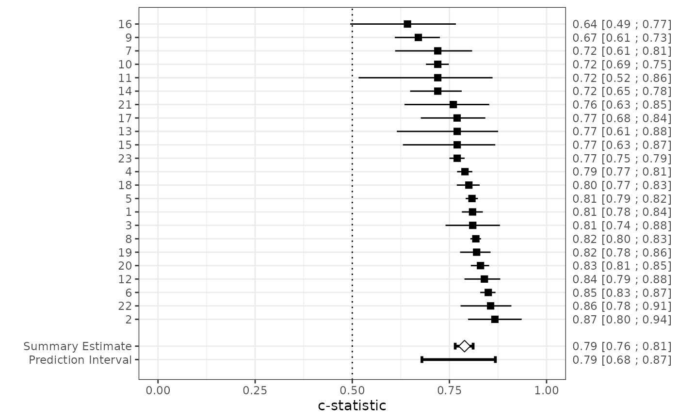
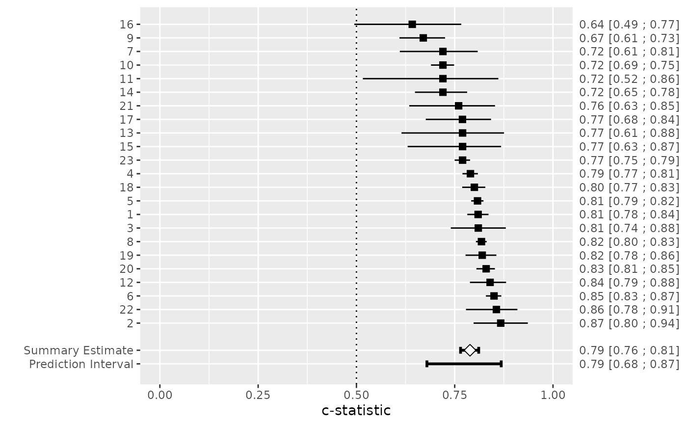
Function to create forest plots for objects of class "valmeta".

Usage

# S3 method for valmeta
plot(x, ...)

Arguments

x

An object of class "valmeta"

...

Additional arguments which are passed to forest.

Value

An object of class ggplot

Details

The forest plot shows the performance estimates of each validation with corresponding confidence intervals. A polygon is added to the bottom of the forest plot, showing the summary estimate based on the model. A 95% prediction interval is added by default for random-effects models, the dotted line indicates its (approximate) bounds.

References

Debray TPA, Damen JAAG, Snell KIE, Ensor J, Hooft L, Reitsma JB, et al. A guide to systematic review and meta-analysis of prediction model performance. BMJ. 2017;356:i6460.

Lewis S, Clarke M. Forest plots: trying to see the wood and the trees. BMJ. 2001; 322(7300):1479--80.

Riley RD, Higgins JPT, Deeks JJ. Interpretation of random effects meta-analyses. BMJ. 2011 342:d549--d549.

See also

When a Bayesian meta-analysis was conducted, the prior and posterior distribution can be visualized using dplot.valmeta. Further, the running means and the presence of autocorrelation can be inspected using rmplot.valmeta and, respectively, acplot.valmeta.

Author

Thomas Debray <thomas.debray@gmail.com>

Examples

data(EuroSCORE)
fit <- valmeta(cstat=c.index, cstat.se=se.c.index, cstat.cilb=c.index.95CIl,
               cstat.ciub=c.index.95CIu, N=n, O=n.events, data=EuroSCORE)
plot(fit)


library(ggplot2)
plot(fit, theme=theme_grey())