Bioequivalence Tests for Parallel Trial Designs: 2 Arms, 1 Endpoint
sampleSize_parallel_2A1E.RmdIn the SimTOST R package, which is specifically designed
for sample size estimation for bioequivalence studies, hypothesis
testing is based on the Two One-Sided Tests (TOST) procedure. (Sozu et al.
2015) In TOST, the equivalence test is framed as a comparison
between the the null hypothesis of ‘new product is worse by a clinically
relevant quantity’ and the alternative hypothesis of ‘difference between
products is too small to be clinically relevant’. This vignette focuses
on a parallel design, with 2 arms/treatments and 1 primary endpoint.
Introduction
Difference of Means Test
This example, adapted from Example 1 in the PASS manual chapter 685 (NCSS 2025), illustrates the process of planning a clinical trial to assess biosimilarity. Specifically, the trial aims to compare blood pressure outcomes between two groups.
Scenario
Drug B is a well-established biologic drug used to control blood pressure. Its exclusive marketing license has expired, creating an opportunity for other companies to develop biosimilars. Drug A is a new competing drug being developed as a potential biosimilar to Drug B. The goal is to determine whether Drug A meets FDA biosimilarity requirements in terms of safety, purity, and therapeutic response when compared to Drug B.
Trial Design
The study follows a parallel-group design with the following key assumptions:
- Reference Group (Drug B): Average blood pressure is 96 mmHg, with a within-group standard deviation of 18 mmHg.
- Mean Difference: As per FDA guidelines, the assumed difference between the two groups is set to mmHg.
- Biosimilarity Limits: Defined as ±1.5σ = ±27 mmHg.
- Desired Type-I Error: 2.5%
- Target Power: 90%
To implement these parameters in R, the following code snippet can be used:
# Reference group mean blood pressure (Drug B)
mu_r <- setNames(96, "BP")

# Treatment group mean blood pressure (Drug A)
mu_t <- setNames(96 + 2.25, "BP")

# Common within-group standard deviation
sigma <- setNames(18, "BP")

# Lower and upper biosimilarity limits
lequi_lower <- setNames(-27, "BP")
lequi_upper <- setNames(27, "BP")
Objective
To explore the power of the test across a range of group sample sizes, power for group sizes varying from 6 to 20 will be calculated.
Implementation
To estimate the power for different sample sizes, we use the sampleSize() function. The
function is configured with a power target of 0.90, a type-I error rate
of 0.025, and the specified mean and standard deviation values for the
reference and treatment groups. The optimization method is set to
"step-by-step" to display the achieved power for each
sample size, providing insights into the results.
Below illustrates how the function can be implemented in R:
library(SimTOST)

(N_ss <- sampleSize(
  power = 0.90,                  # Target power
  alpha = 0.025,                 # Type-I error rate
  mu_list = list("R" = mu_r, "T" = mu_t), # Means for reference and treatment groups
  sigma_list = list("R" = sigma, "T" = sigma), # Standard deviations
  list_comparator = list("T_vs_R" = c("R", "T")), # Comparator setup
  list_lequi.tol = list("T_vs_R" = lequi_lower),  # Lower equivalence limit
  list_uequi.tol = list("T_vs_R" = lequi_upper),  # Upper equivalence limit
  dtype = "parallel",            # Study design
  ctype = "DOM",                 # Comparison type
  lognorm = FALSE,               # Assumes normal distribution
  optimization_method = "step-by-step", # Optimization method
  ncores = 1,                    # Single-core processing
  nsim = 1000,                   # Number of simulations
  seed = 1234                    # Random seed for reproducibility
))
#> Sample Size Calculation Results
#> -------------------------------------------------------------
#> Study Design: parallel trial targeting 90% power with a 2.5% type-I error.
#>
#> Comparisons:
#>    R vs. T
#>     - Endpoints Tested: BP
#> -------------------------------------------------------------
#>                  Parameter       Value
#>          Total Sample Size          26
#>             Achieved Power        90.8
#>  Power Confidence Interval 88.8 - 92.5
#> -------------------------------------------------------------

# Display iteration results
N_ss$table.iter
#> Index: <n_iter>
#>     n_iter n_drop   n_R   n_T n_total power  power_LCI  power_UCI
#>      <int>  <num> <num> <num>   <num> <num>      <num>      <num>
#>  1:      2      0     2     2       4 0.042 0.03079269 0.05685194
#>  2:      3      0     3     3       6 0.071 0.05622292 0.08916283
#>  3:      4      0     4     4       8 0.118 0.09898992 0.14000650
#>  4:      5      0     5     5      10 0.197 0.17305355 0.22331236
#>  5:      6      0     6     6      12 0.335 0.30593958 0.36534479
#>  6:      7      0     7     7      14 0.468 0.43675913 0.49948974
#>  7:      8      0     8     8      16 0.597 0.56577960 0.62746582
#>  8:      9      0     9     9      18 0.698 0.66831899 0.72613905
#>  9:     10      0    10    10      20 0.766 0.73825476 0.79167071
#> 10:     11      0    11    11      22 0.828 0.80284126 0.85059491
#> 11:     12      0    12    12      24 0.885 0.86320172 0.90377751
#> 12:     13      0    13    13      26 0.908 0.88794993 0.92484078
We can visualize the power curve for a range of sample sizes using the following code snippet:
plot(N_ss)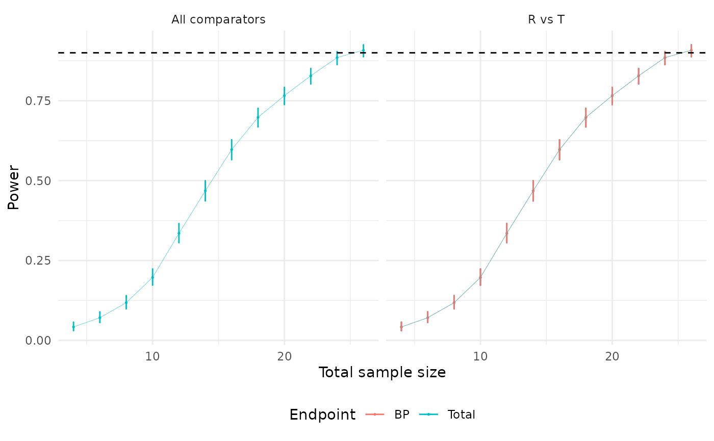
To account for an anticipated dropout rate of 20% in each group, we need to adjust the sample size. The following code demonstrates how to incorporate this adjustment using a custom optimization routine. This routine is designed to find the smallest integer sample size that meets or exceeds the target power. It employs a stepwise search strategy, starting with large step sizes that are progressively refined as the solution is approached.
# Adjusted sample size calculation with 20% dropout rate
(N_ss_dropout <- sampleSize(
  power = 0.90,                  # Target power
  alpha = 0.025,                 # Type-I error rate
  mu_list = list("R" = mu_r, "T" = mu_t), # Means for reference and treatment groups
  sigma_list = list("R" = sigma, "T" = sigma), # Standard deviations
  list_comparator = list("T_vs_R" = c("R", "T")), # Comparator setup
  list_lequi.tol = list("T_vs_R" = lequi_lower),  # Lower equivalence limit
  list_uequi.tol = list("T_vs_R" = lequi_upper),  # Upper equivalence limit
  dropout = c("R" = 0.20, "T" = 0.20), # Expected dropout rates
  dtype = "parallel",            # Study design
  ctype = "DOM",                 # Comparison type
  lognorm = FALSE,               # Assumes normal distribution
  optimization_method = "fast",  # Fast optimization method
  nsim = 1000,                   # Number of simulations
  seed = 1234                    # Random seed for reproducibility
))
#> Sample Size Calculation Results
#> -------------------------------------------------------------
#> Study Design: parallel trial targeting 90% power with a 2.5% type-I error.
#>
#> Comparisons:
#>    R vs. T
#>     - Endpoints Tested: BP
#> -------------------------------------------------------------
#>                  Parameter       Value
#>          Total Sample Size          32
#>             Achieved Power        90.8
#>  Power Confidence Interval 88.8 - 92.5
#> -------------------------------------------------------------
Previously, finding the required sample size took 12 iterations. With the custom optimization routine, the number of iterations was reduced to 8, significantly improving efficiency.