Imputation via Joint Modelling
Imputation via Joint Modelling
![]()
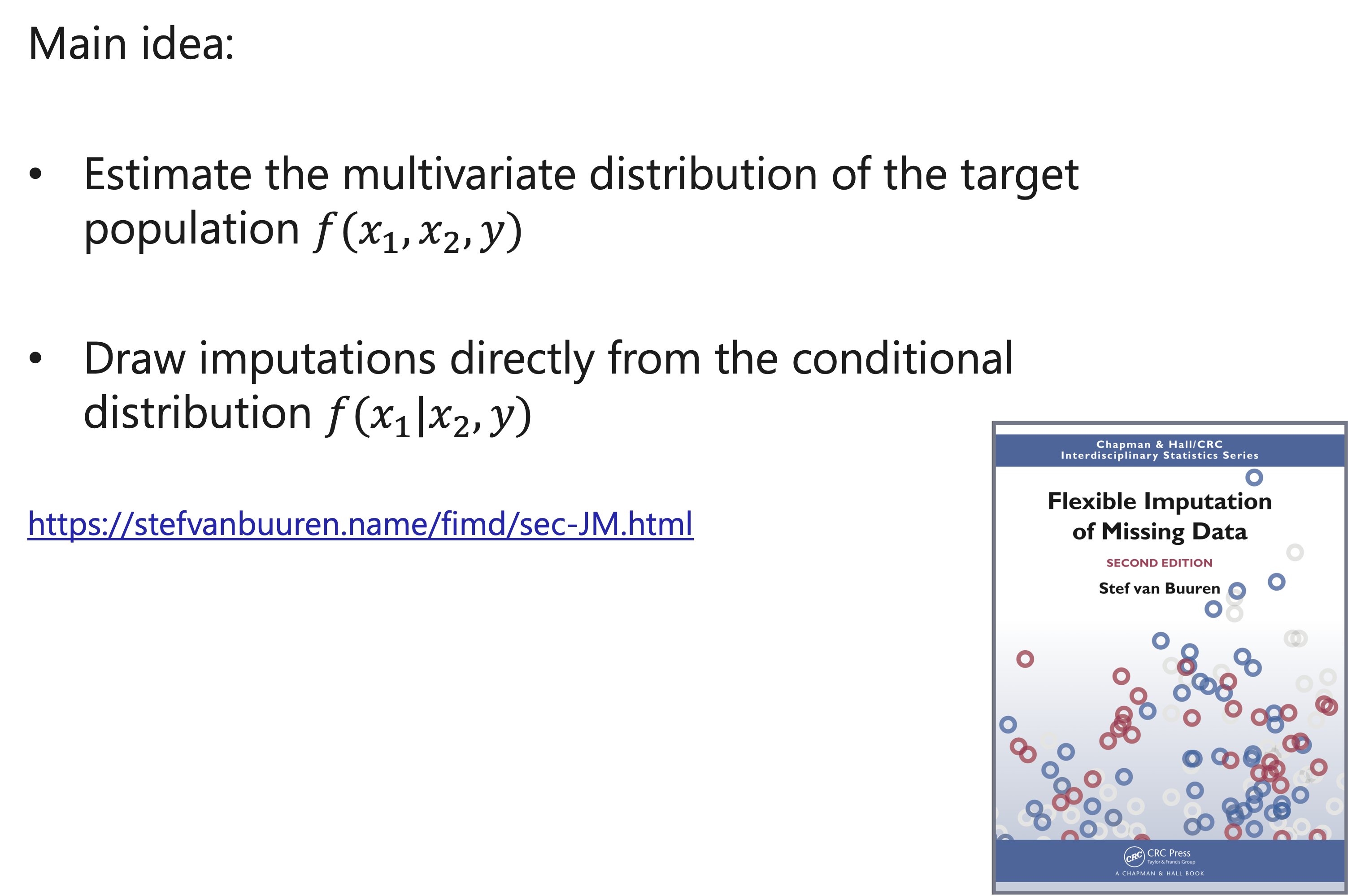
Imputation via Joint Modelling
It is common to assume that all data follow a multivariate Normal or Student-T distribution
\((𝑥_1,𝑥_2,𝑦) \sim MVN (𝜇,"Σ" )\)
For now, we consider that
- The mean vector μ is known
- The covariance matrix Σ is known
Imputation via Joint Modelling
![]()
Imputation via Joint Modelling
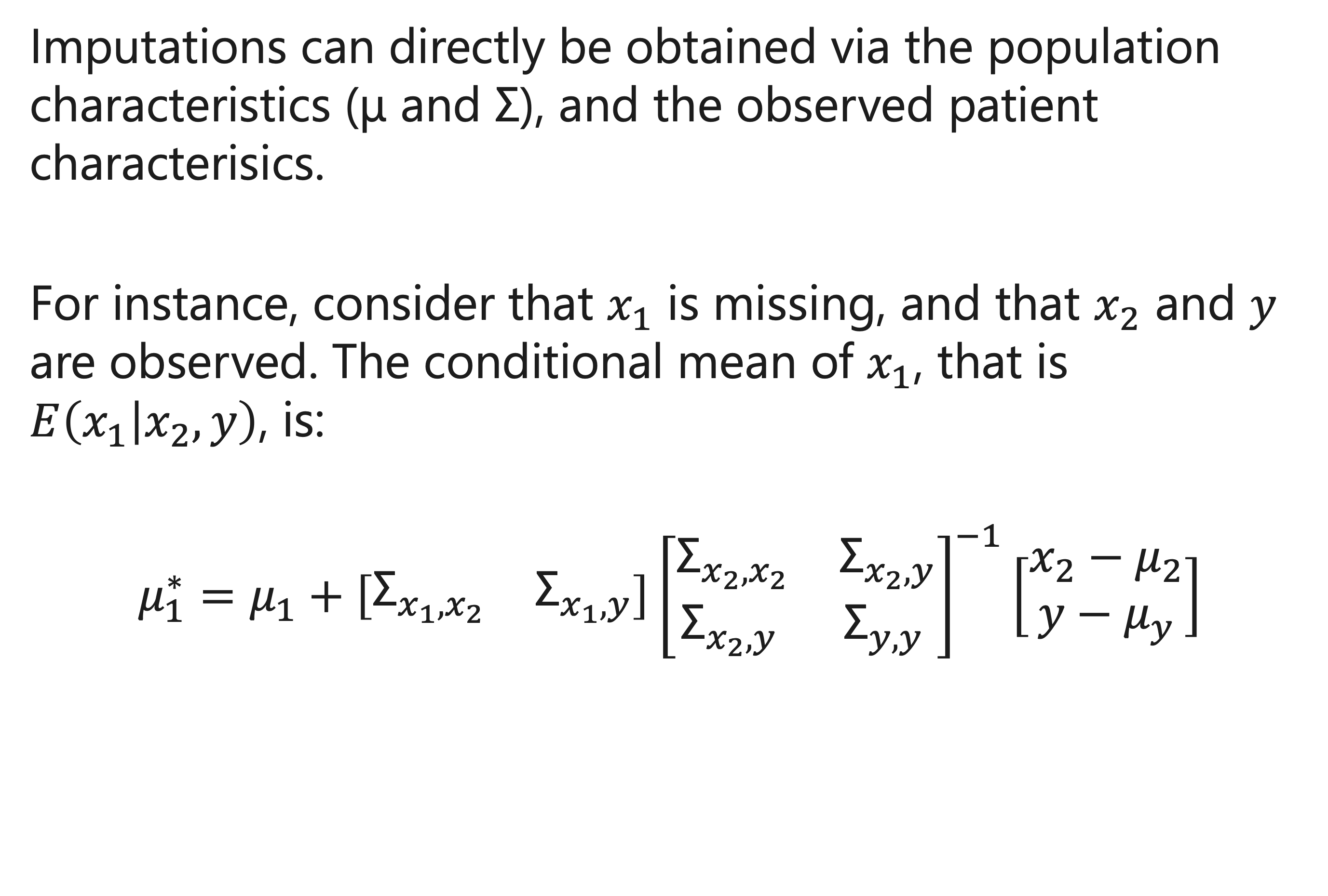
How to use the conditional mean?
\(𝜇_1^∗\) is the most likely value for \(𝑥_1\), and can thus be used as imputation.
\(𝜇_1^∗\) is equal to the mean of \(𝑥_1\) plus an adjustment.
- If there is little correlation between the predictors and outcomes, then the best guess for \(𝑥_1\) is the mean of \(𝑥_1\).
Imputation via Joint Modelling
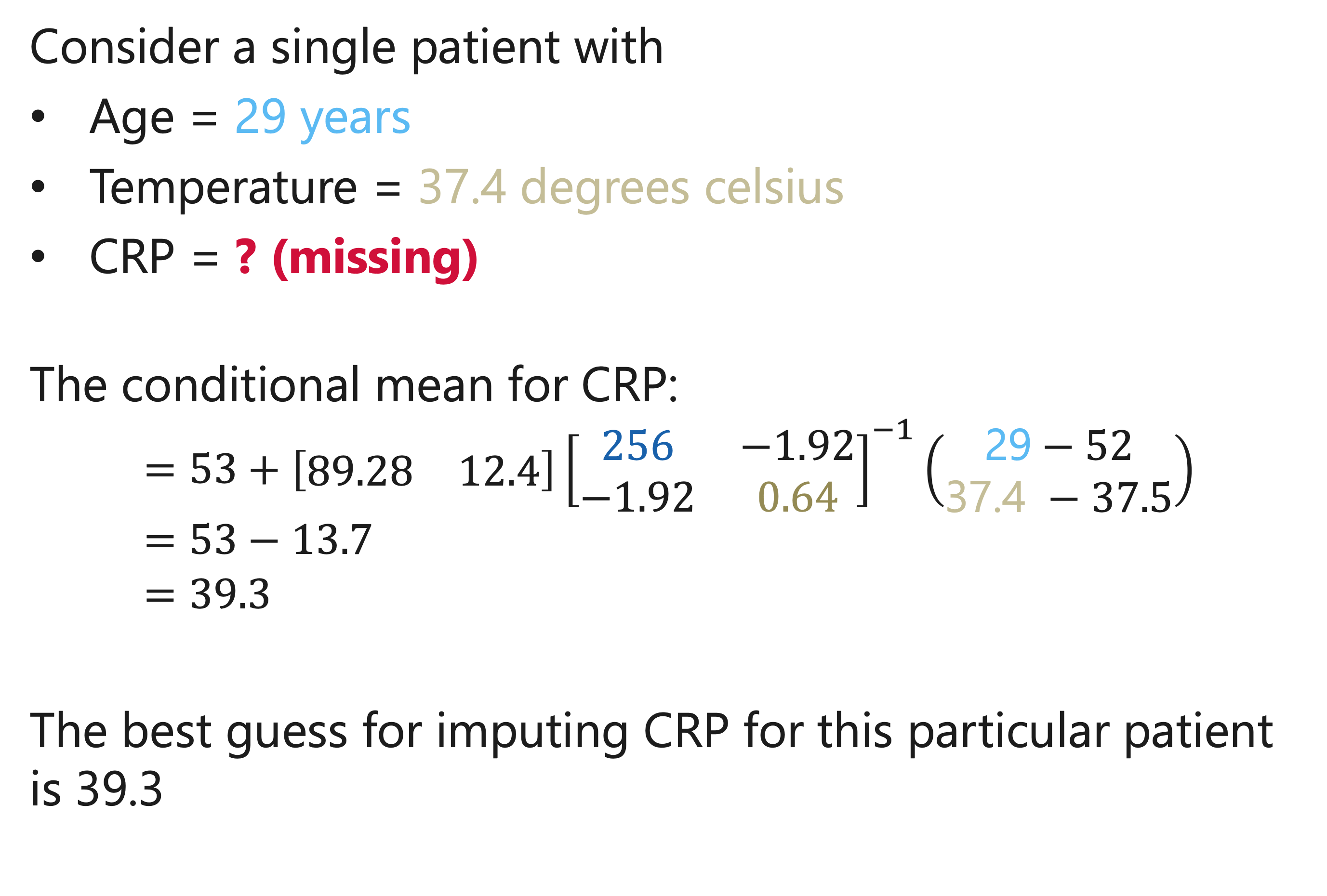
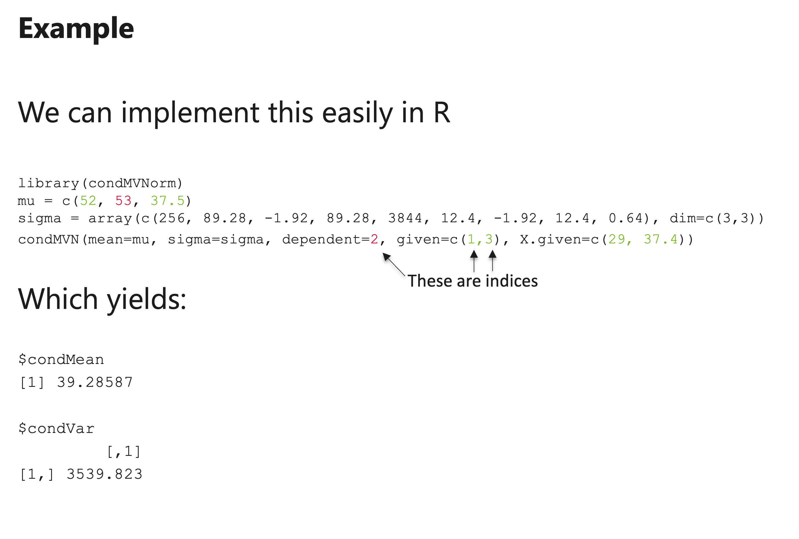
Example
Multivariate distribution of patients presenting with lower respiratory tract infections in primary care:
- Age, years: mean = 52, SD = 16
- C-reactive protein: mean = 53, SD = 62
- Temperature, C°: mean = 37.5, SD = 0.8
- Cor (Age, CRP) = 0.09
- Cor(Age, Temperature) = -0.15
- Cor(CRP, Temperature) = 0.25
Imputation via Joint Modelling
![]()
Imputation via Joint Modelling
![]()
Imputation via Joint Modelling
![]()
Imputation via Joint Modelling
![]()
Imputation via Joint Modelling
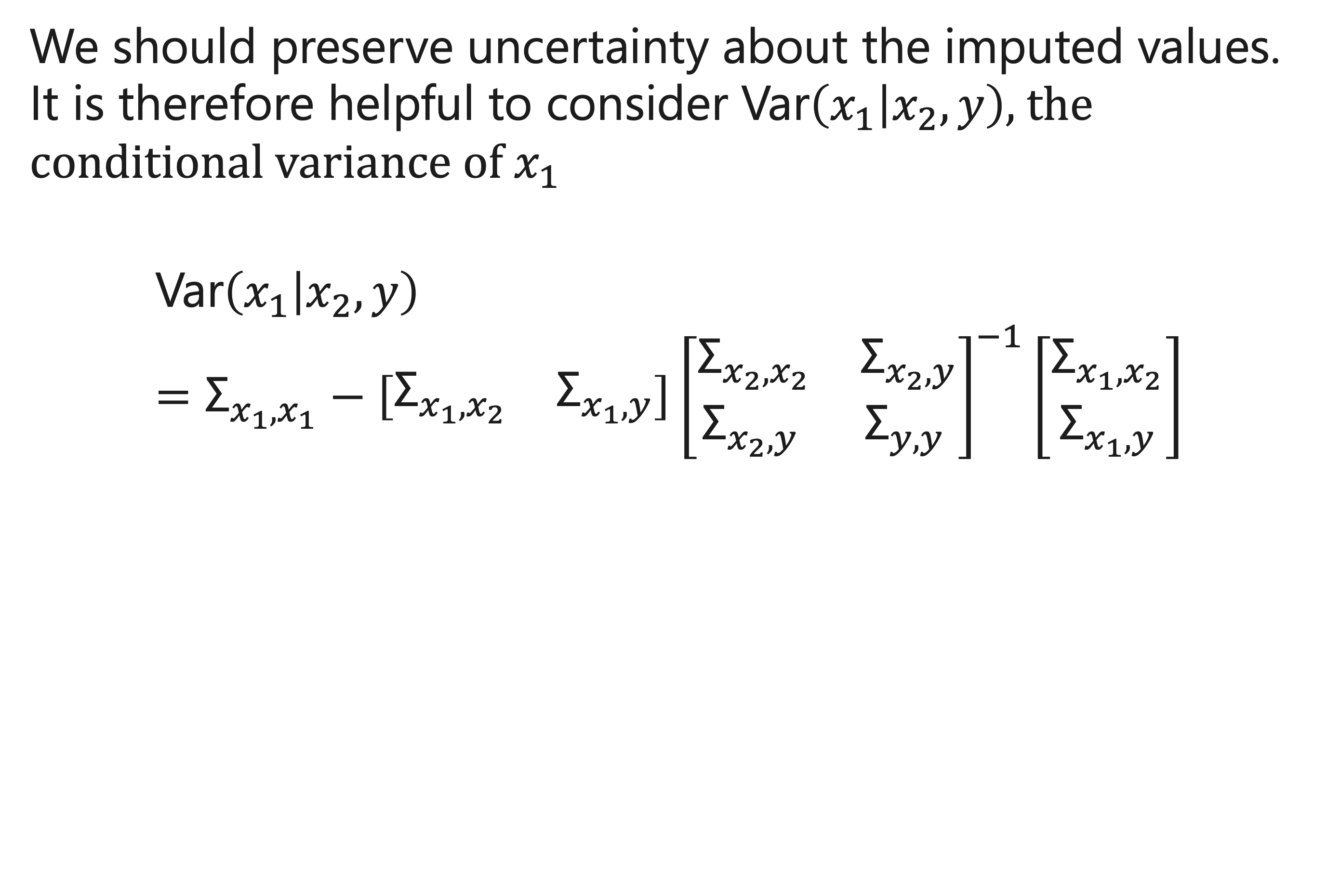
How to use the conditional variance?
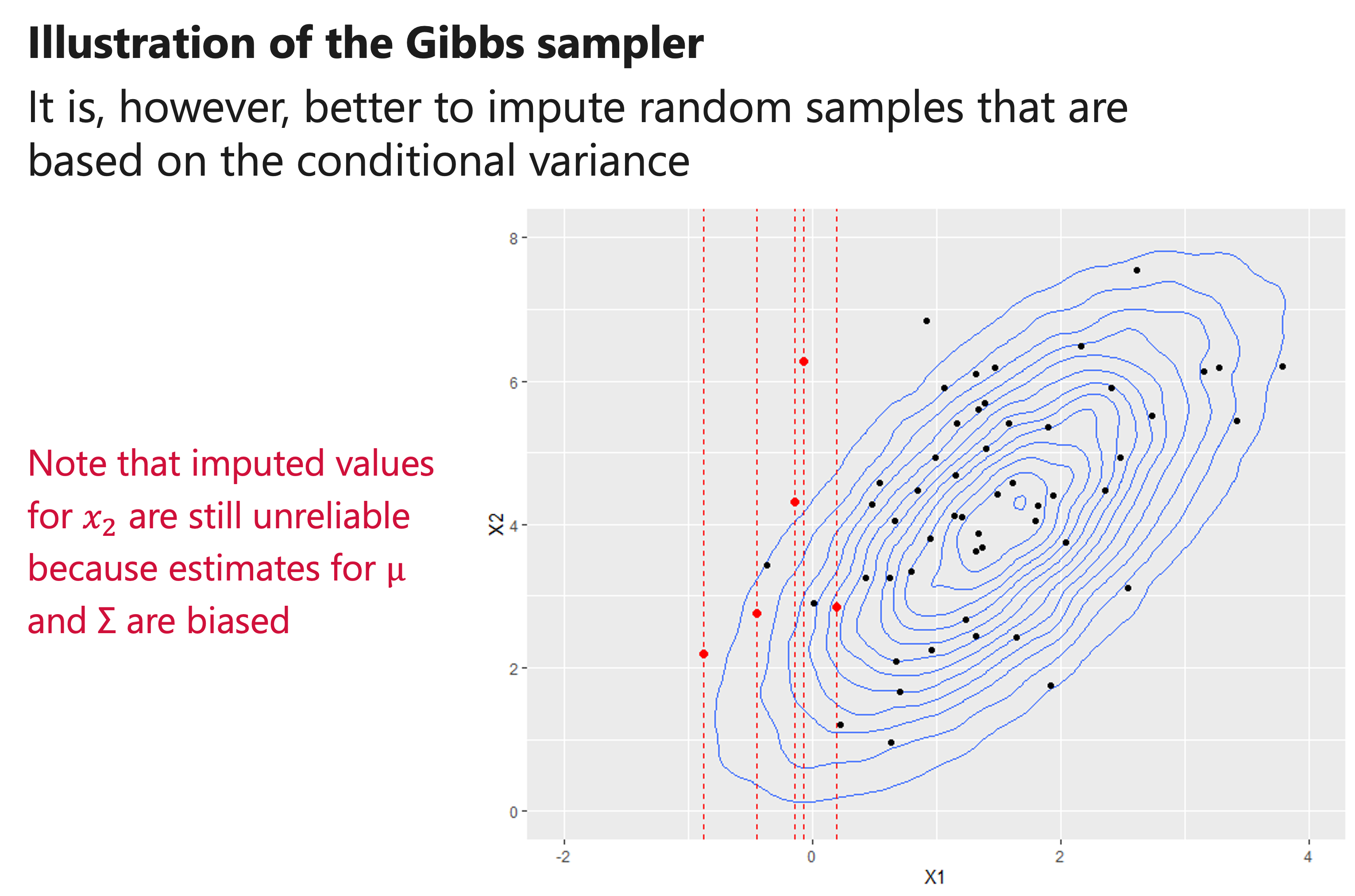
“Var” \((𝑥_1│𝑥_2, 𝑦)\) quantifies the variance of \(𝜇_1^∗\) , and can be used to draw multiple imputations. In particular, we can sample an imputed value from a Normal distribution with mean \(𝜇_1^∗\) and variance “Var” \((𝑥_1│𝑥_2, 𝑦)\)
“Var” \((𝑥_1│𝑥_2, 𝑦)\) is equal to the variance of \(𝑥_1\) minus an adjustment. If there is little correlation between the predictors and outcomes, then the variance of imputed values for \(𝑥_1\) is equal to the variance of \(𝑥_1\) in the original population.
Imputation via Joint Modelling
![]()
Imputation via Joint Modelling
![]()
Imputation via Joint Modelling
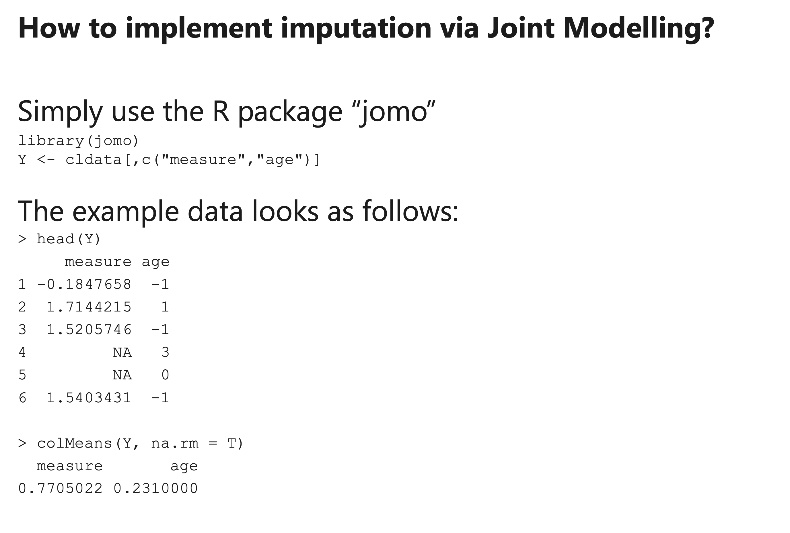
So, how to generate an imputed dataset?
An iterative procedure is needed:
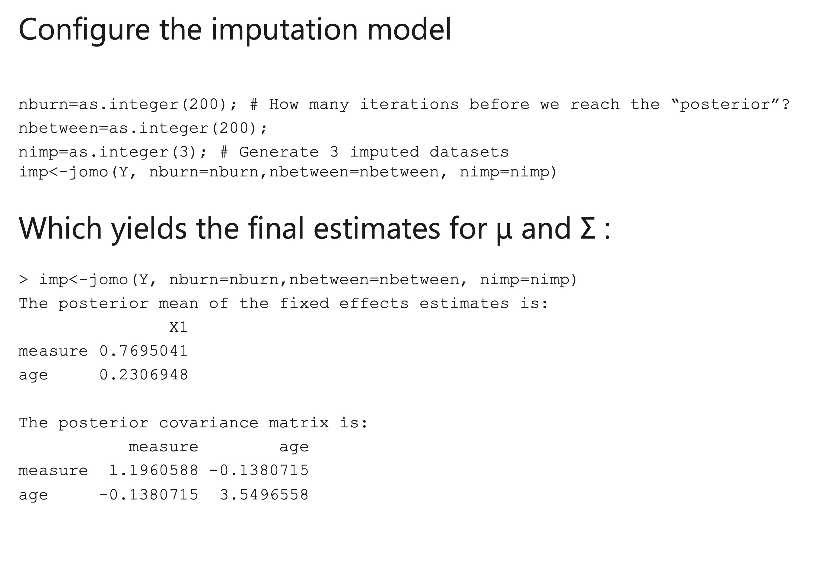
- Estimate μ and Σ
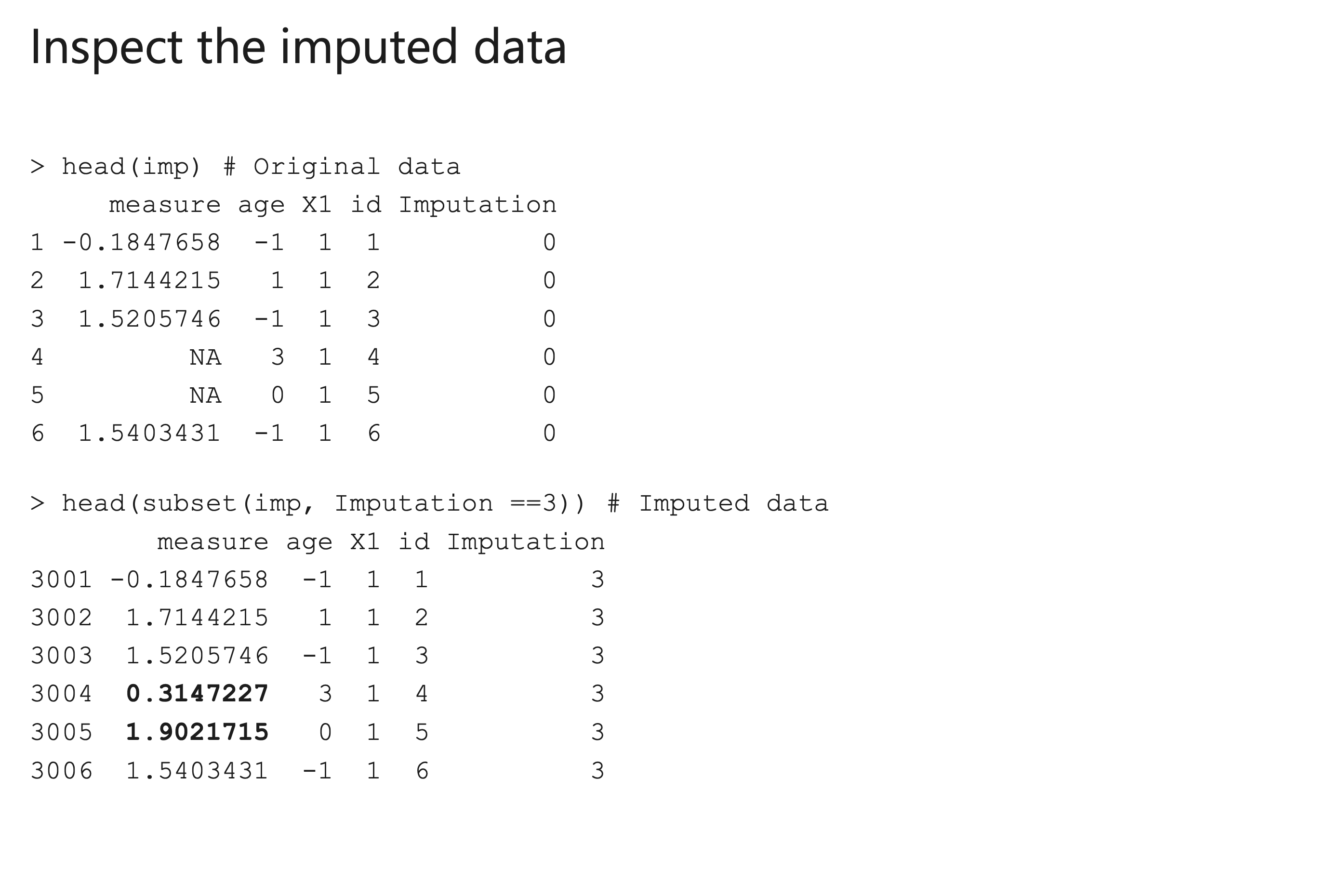
- Use μ and Σ to impute the missing values
- Update estimates of μ and Σ using the imputed values
- Continue until estimates of μ and Σ stabilize
This approach is known as the Gibbs sampler
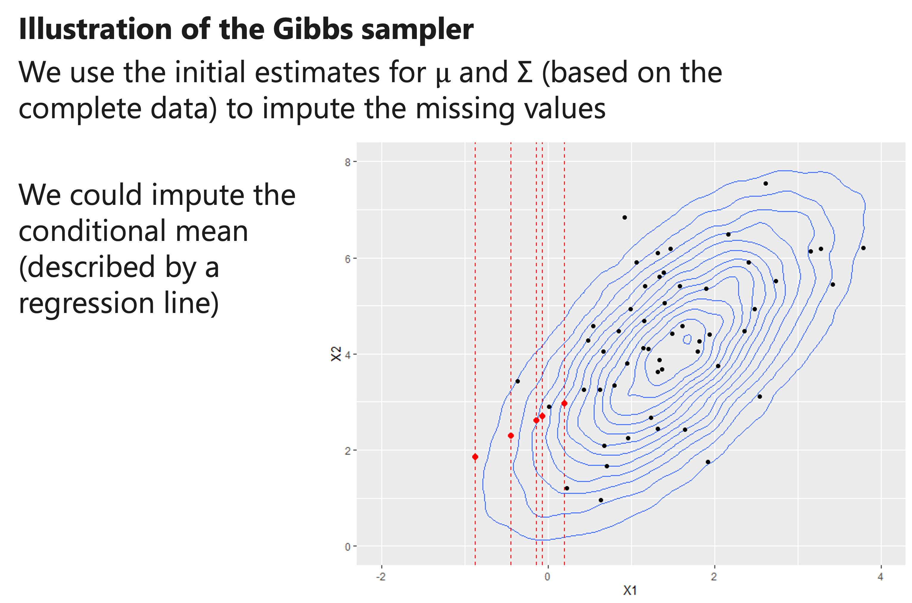
A natural choice for the initial estimates of μ and Σ is to derive them directly using the complete data only.
Imputation via Joint Modelling
![]()
Imputation via Joint Modelling
![]()
Imputation via Joint Modelling
![]()
Imputation via Joint Modelling
![]()
Imputation via Joint Modelling
![]()
Imputation via Joint Modelling
![]()
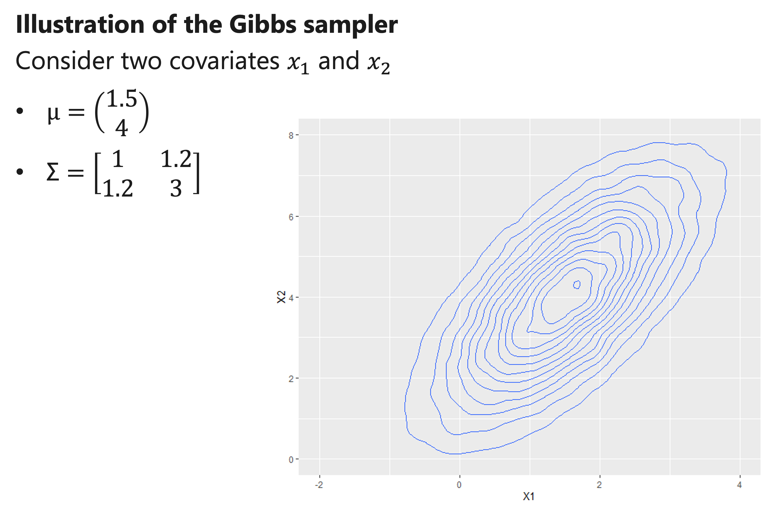
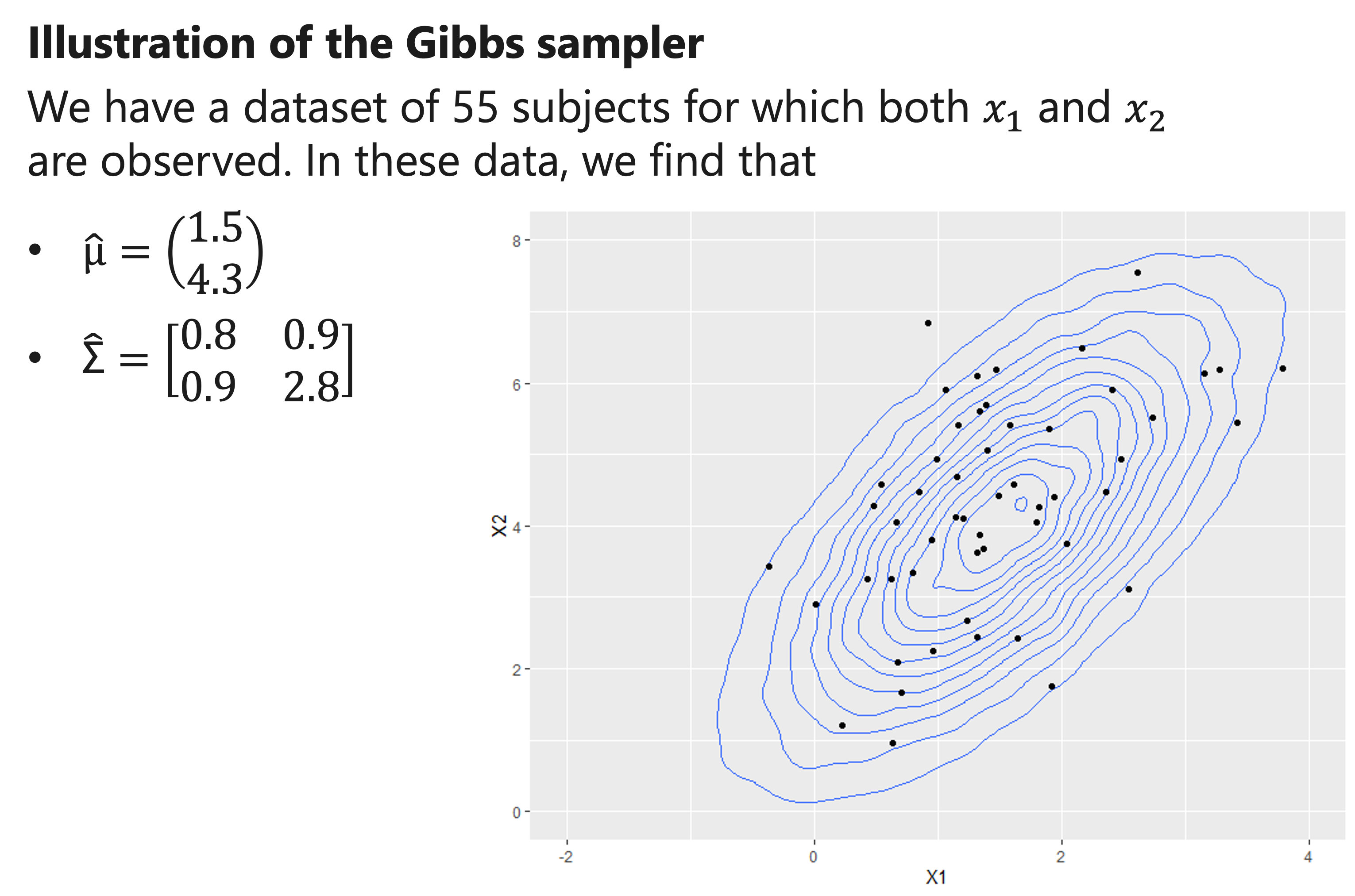
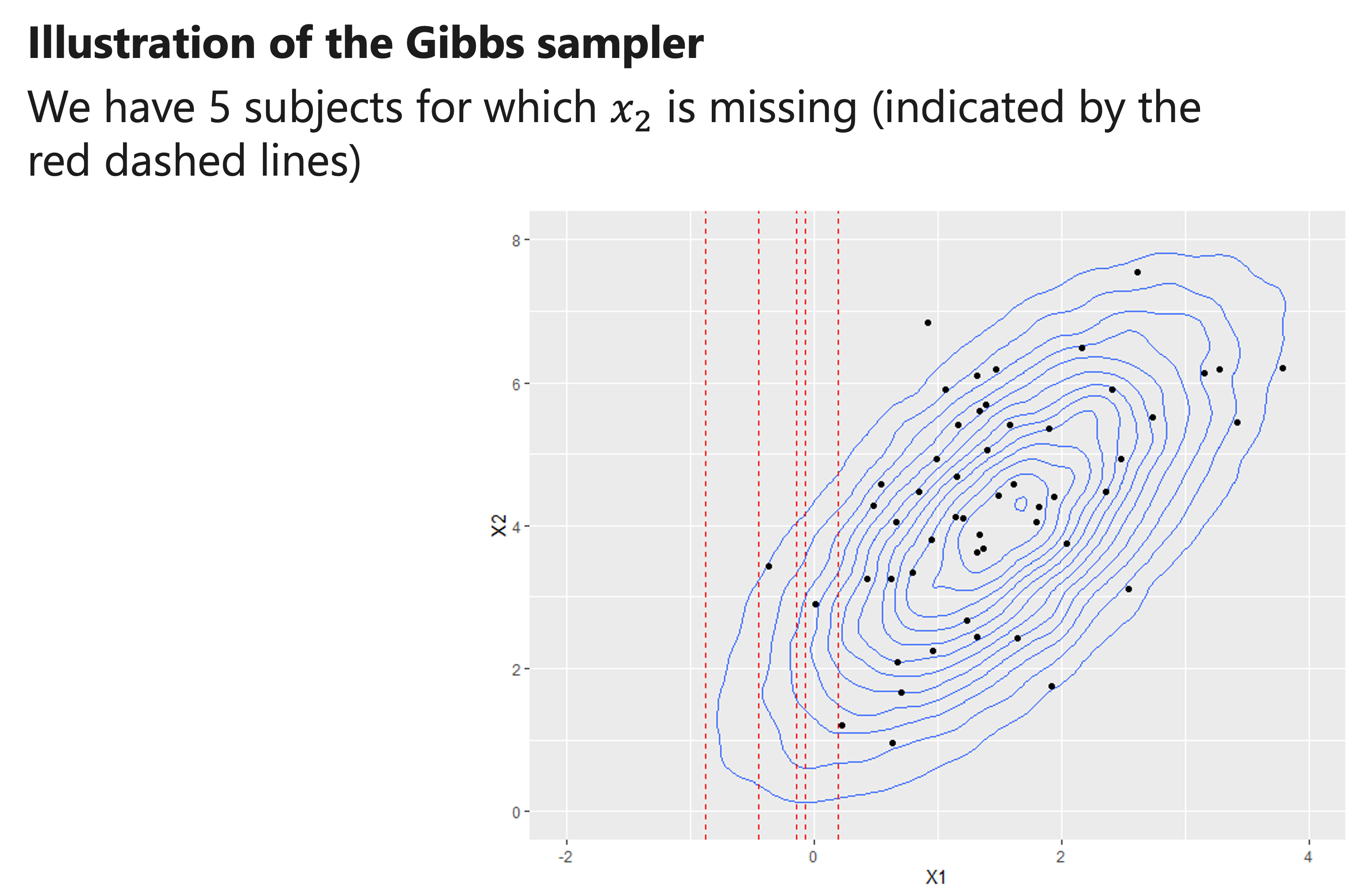
Imputation via Joint Modelling
Illustration of the Gibbs sampler
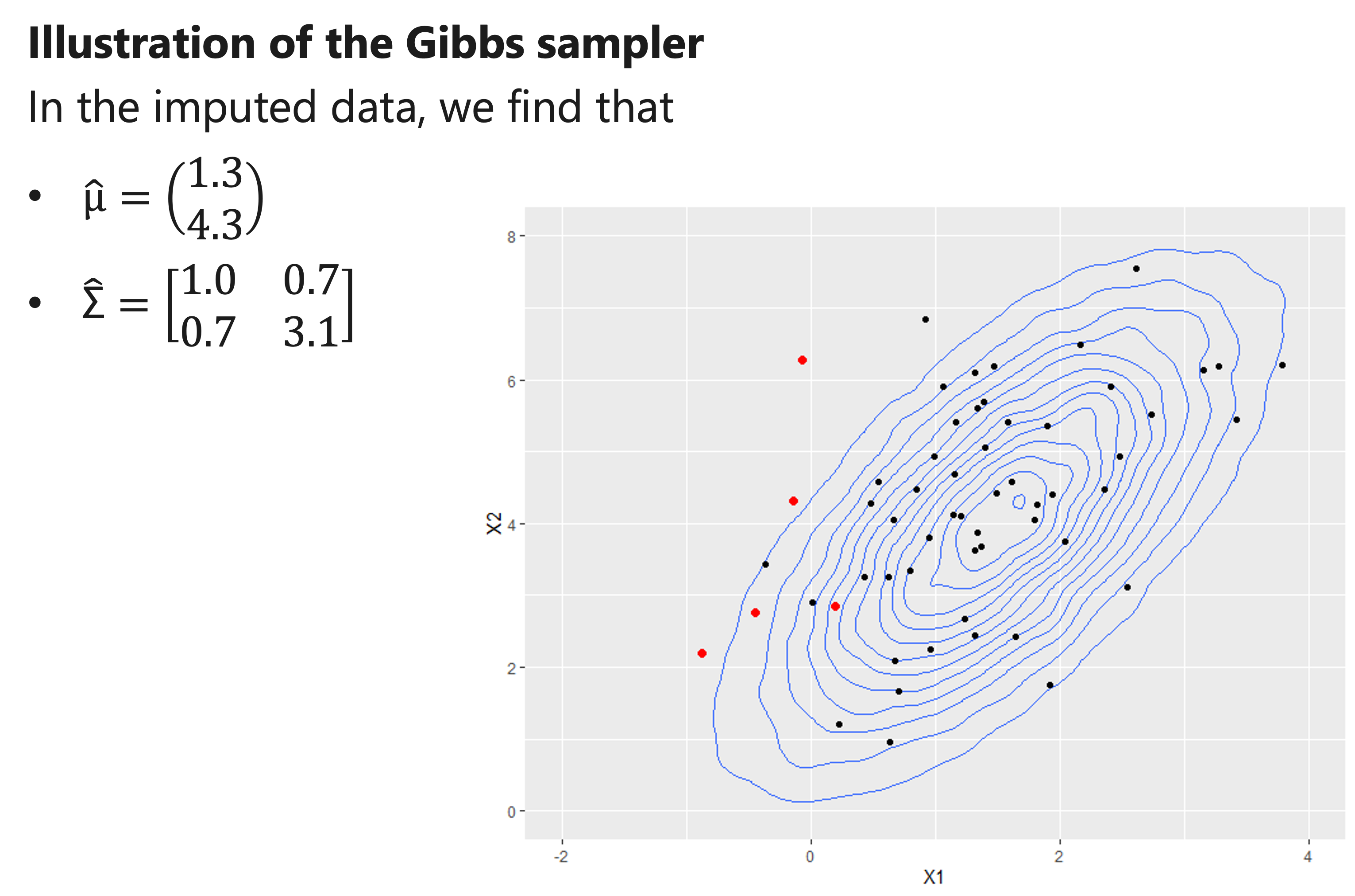
- We impute missing values using the new estimates for μ and “Σ”, and re-estimate μ and “Σ” .
- We iterate this procedure many times.
- Eventually, we should obtain reliable estimates for μ and “Σ” , and thus also obtain imputations that properly reflect their uncertainty
Imputation via Joint Modelling
![]()
Imputation via Joint Modelling
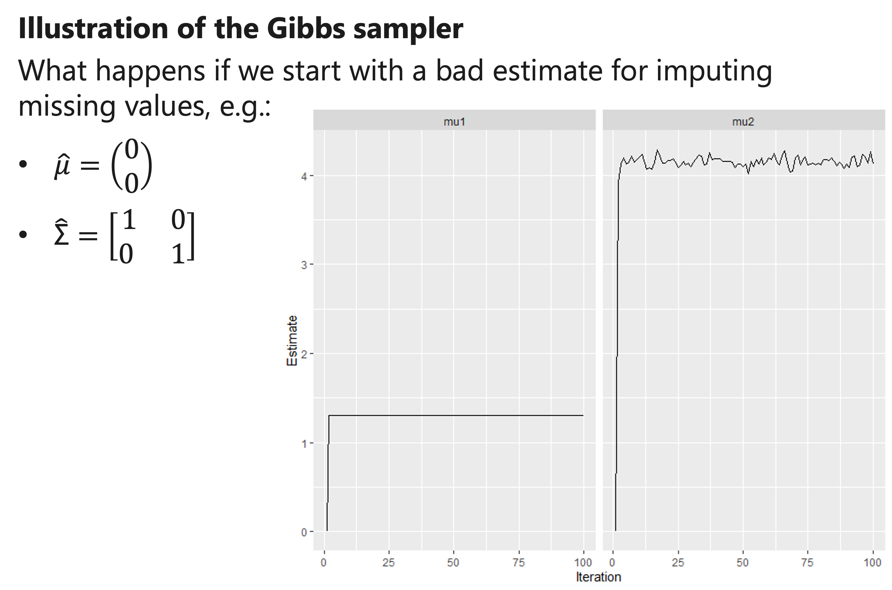
How to ensure that we end up in the posterior distribution?
Imputation via Joint Modelling
![]()
Imputation via Joint Modelling
![]()
Imputation via Joint Modelling
![]() ## Imputation via Joint Modelling
## Imputation via Joint Modelling
Imputation via Joint Modelling
Final considerations


 ## Imputation via Joint Modelling